Annotation
Being skilled at identifying vulnerabilities in source code, executing SQL injection attack, exploiting outdated services in well-known scripts, and even infiltrating enterprises to gain access to Domain admin privileges are valuable abilities for someone with a hacker mindset.But is it enough if you want to be a Red Teamer and cover all the 7 Defense in Depth layers?
To reduce the gaps, today we will talk about breaching the physical perimeter, tricking security guards, control gates and barriers remotely and Software Defined Radio represented by HackRF will help us in that.
0. What is HackRF
HackRF (https://greatscottgadgets.com/hackrf/one/) is a versatile software-defined radio (SDR) platform that allows users to explore and experiment with radio frequencies. It was created by Michael Ossmann (https://twitter.com/michaelossmann) and is designed to be an affordable and accessible tool for radio frequency (RF) research and development.
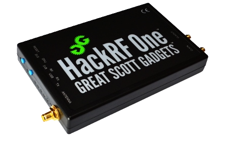
The HackRF hardware consists of a small, portable device that connects to a computer via USB. It is equipped with a wideband RF transceiver that can transmit and receive signals across a broad frequency range, typically from 1 MHz to 6 GHz (my Spectrum Analyzer allows me to perform till 7,25 GHz). This flexibility enables to work with various wireless protocols, such as Wi-Fi, Bluetooth, GSM, RFID, and more.
One of the main features of HackRF is its ability to operate as a fully programmable radio. It is controlled by software running on a host computer, which allows to manipulate and analyze signals in real-time. The device provides access to raw radio signals, enabling tasks such as signal capture, demodulation, spectrum analysis, and protocol decoding.
HackRF’s open-source nature and extensive software support make it a popular choice among security professionals and hackers (not by its name, but because of its features:)). The device is compatible with a wide range of software tools and libraries, including GNU Radio, an open-source signal processing framework (we will talk about that later).
HackRF is often compared with other hardware “toys” like FlipperZero and RTL-SDR due to their similar features. Indeed, all of them can work with RF, but…
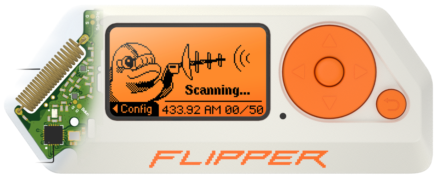
FlipperZero can receive and transmit radio frequencies as well as HackRF, but the range is limited by 300-348 MHz, 387-464 MHz, and 779-928 MHz bands (overall 274 MHZ range or 4,5% of HackRF). Moreover, the antenna is quite short, small and inside the device hence we can forget about long distance communications.
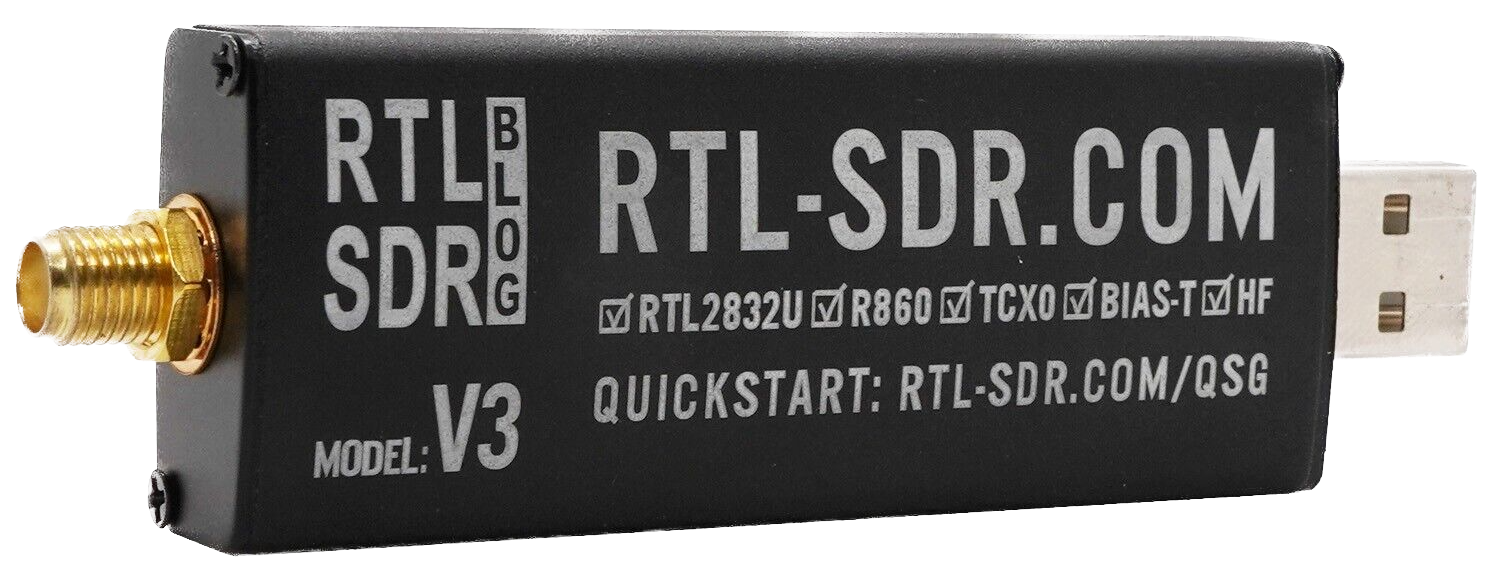
RTL-SDR, depending on the particular model, could receive frequencies from 500 kHz up to 1.75 GHz (30% of HackRF). You can use the external antenna, connect the dongle directly to PC and work with the same apps like HackRF does. Also, it’s the price reasonable device – the official price is $33 (unlike $300+ for HackRF). But it has one major drawback – RTL-SDR can’t transmit the signals. Which means you can only “hear”, but not “talk”.
1. The equipment
Allow us to share our journey with HackRF, including the challenges we encountered and how we effectively resolve them. We believe that our insights can save you significant time and resources. Let’s get started.
A. HackRF
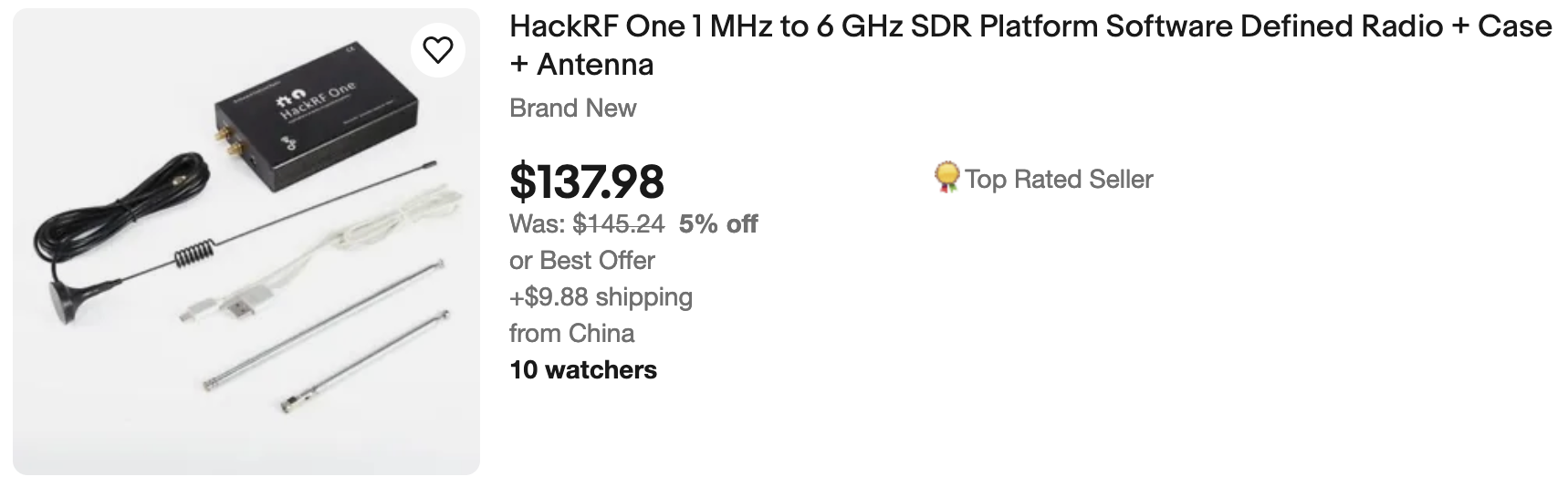
We purchased the HackRF One with some addons: 3.2 inch LCD Portapack H2 and Aluminum Case Battery. The overall price was $200.
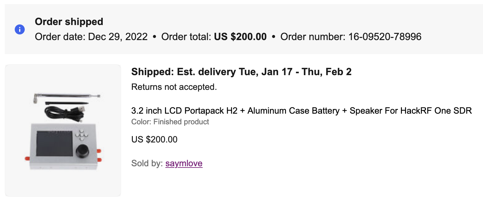
The delivery was quicker than expected, arriving in just one month instead of the initially estimated two months as mentioned in the description. The package was in excellent condition and the device functioned perfectly. One of the standout features of the PortaPack add-on is its standalone usability, allowing you to operate it independently without needing to connect it to a laptop.
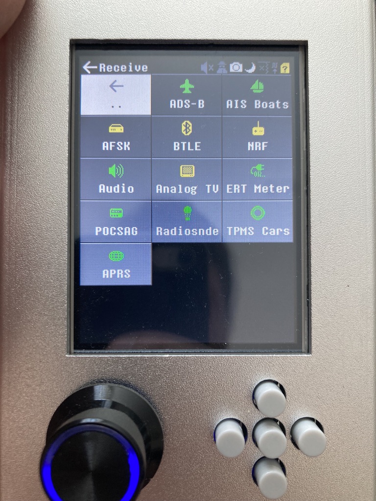
It comes equipped with a battery, SD-card slot, and preset frequencies. While it’s possible to connect this device to a PC and utilize it as a regular HackRF, you need to activate a specific mode for this purpose. After using this assembly for a period, we found it to be rather impractical, especially for our needs. To begin with, the battery life doesn’t exceed 10-15 minutes. As a result, you might have noticed in YouTube videos that the PortaPack is connected to a Power Bank for extended use. Furthermore, in terms of hacking capabilities, it can only execute Replay attacks. Additionally, as previously mentioned, if you intend to use it with a PC, you have to manually switch to HackRF mode each time, which is considerably inconvenient. Lastly, its size is notable, being 2-3 times wider than a single HackRF device.
Keeping that in mind, we decided to disassemble the device and keep only the HackRF.
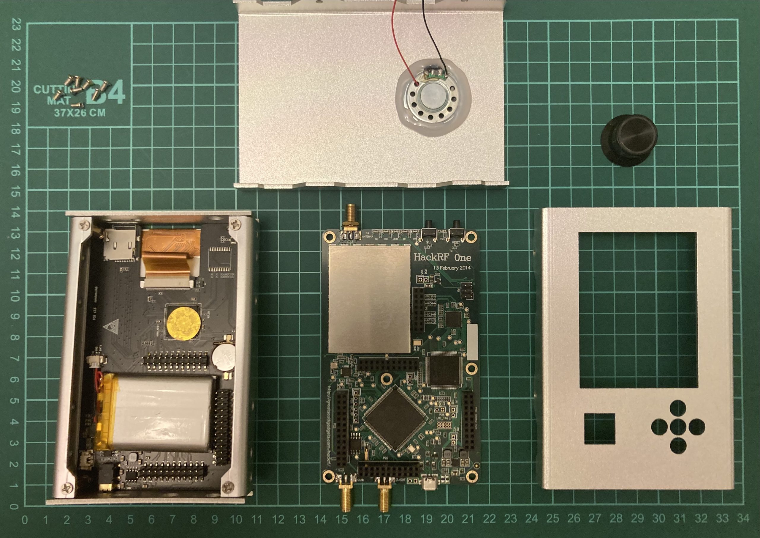
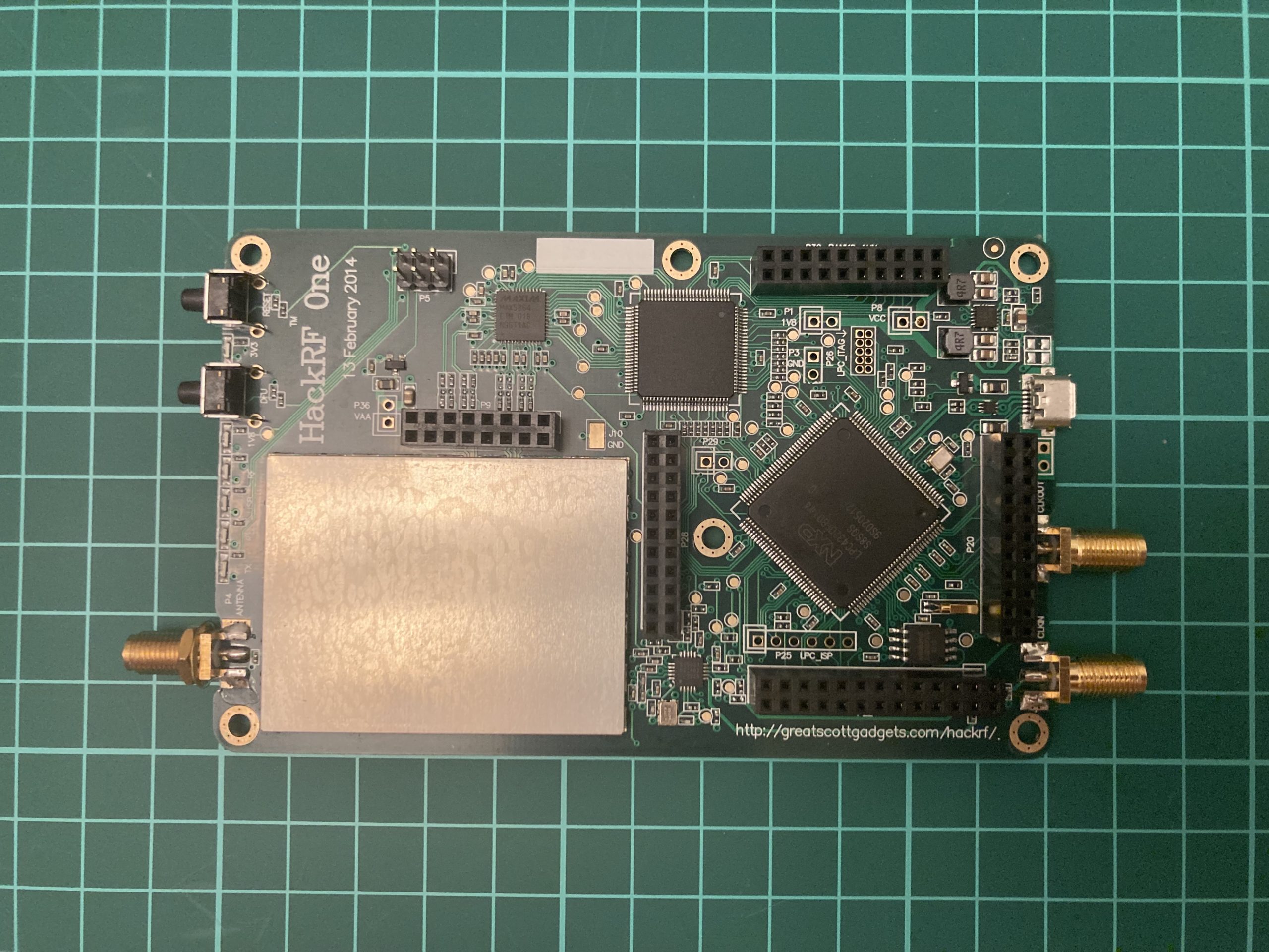
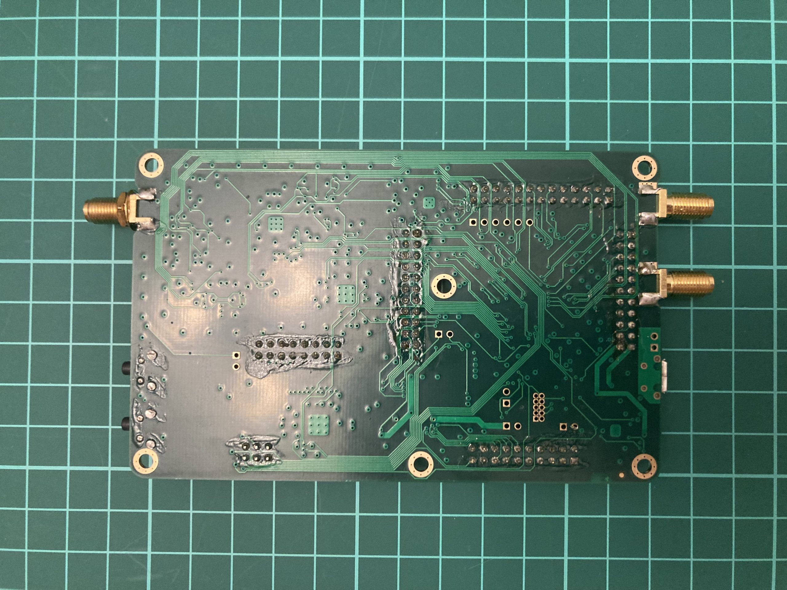
The HackRF circuit board, in comparison to the entire device, is relatively slim and lightweight, making it quite functional as it is – simply plug in the antenna and connect the USB cable to your PC. I’d like to draw your attention to the lower left corner of the image, where you can see a gray rectangle with a yellow line on its side, encircled by pins. This component represents the battery. This insight sheds light on why the lifespan of the HackRF + PortaPack combination is notably limited.
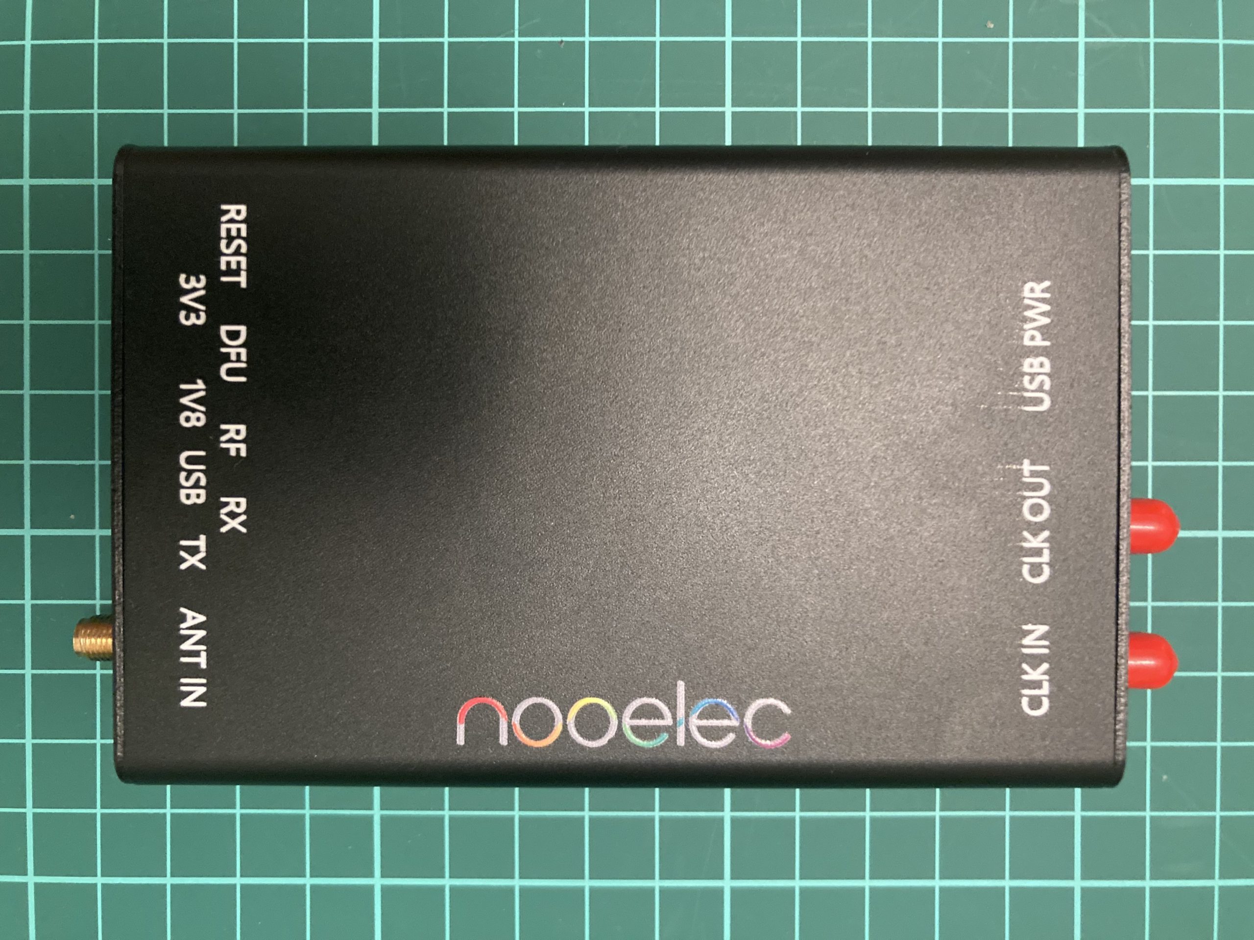
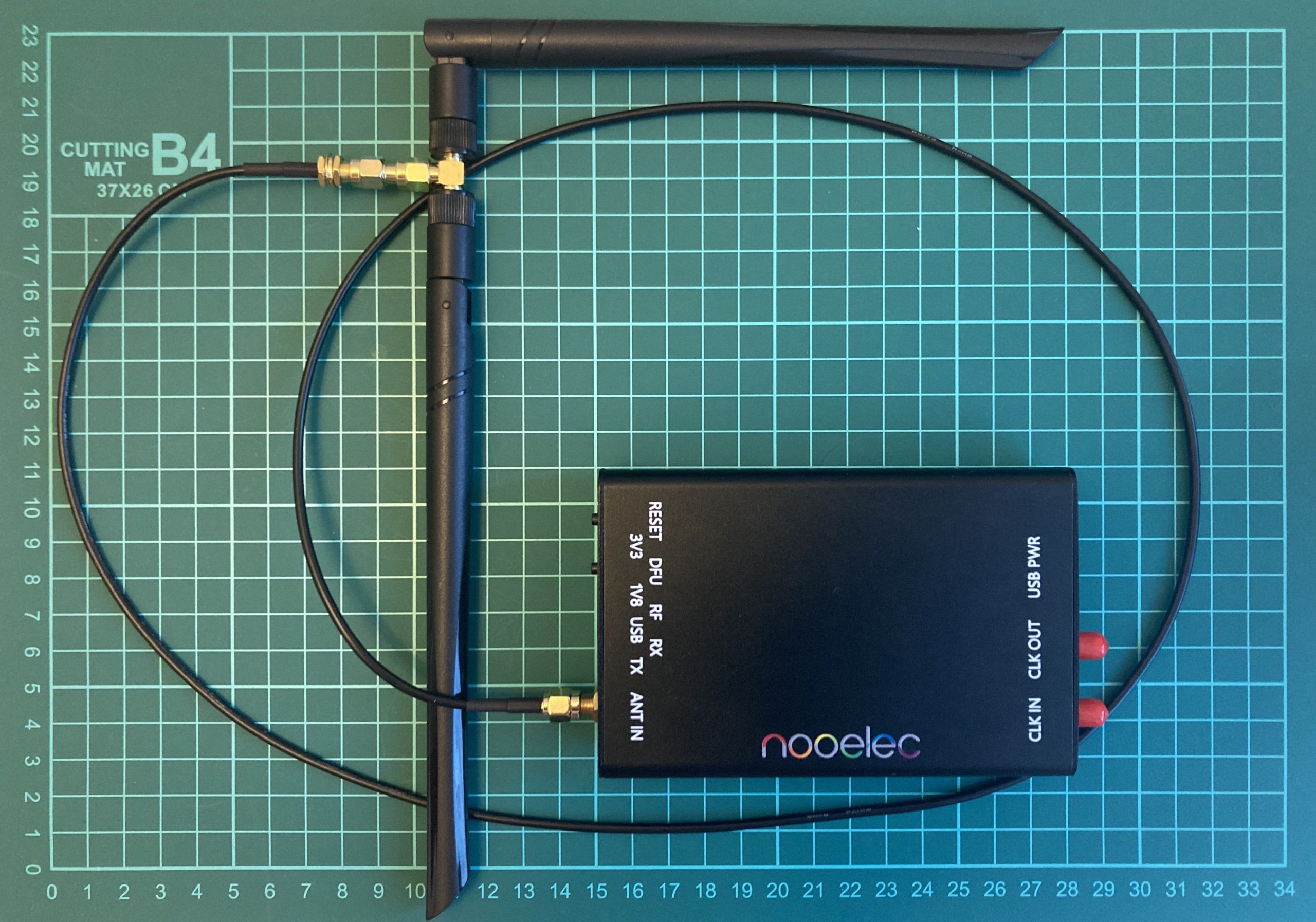
To keep the HackRF safe and protect from the external damage, we ordered the Nooelec case (about $28 + $12 shipping). It’s an aluminum body 2 centimeters height, 8 cm wide and 12,5 cm length with matching holes under the LED and USB and SMA ports.
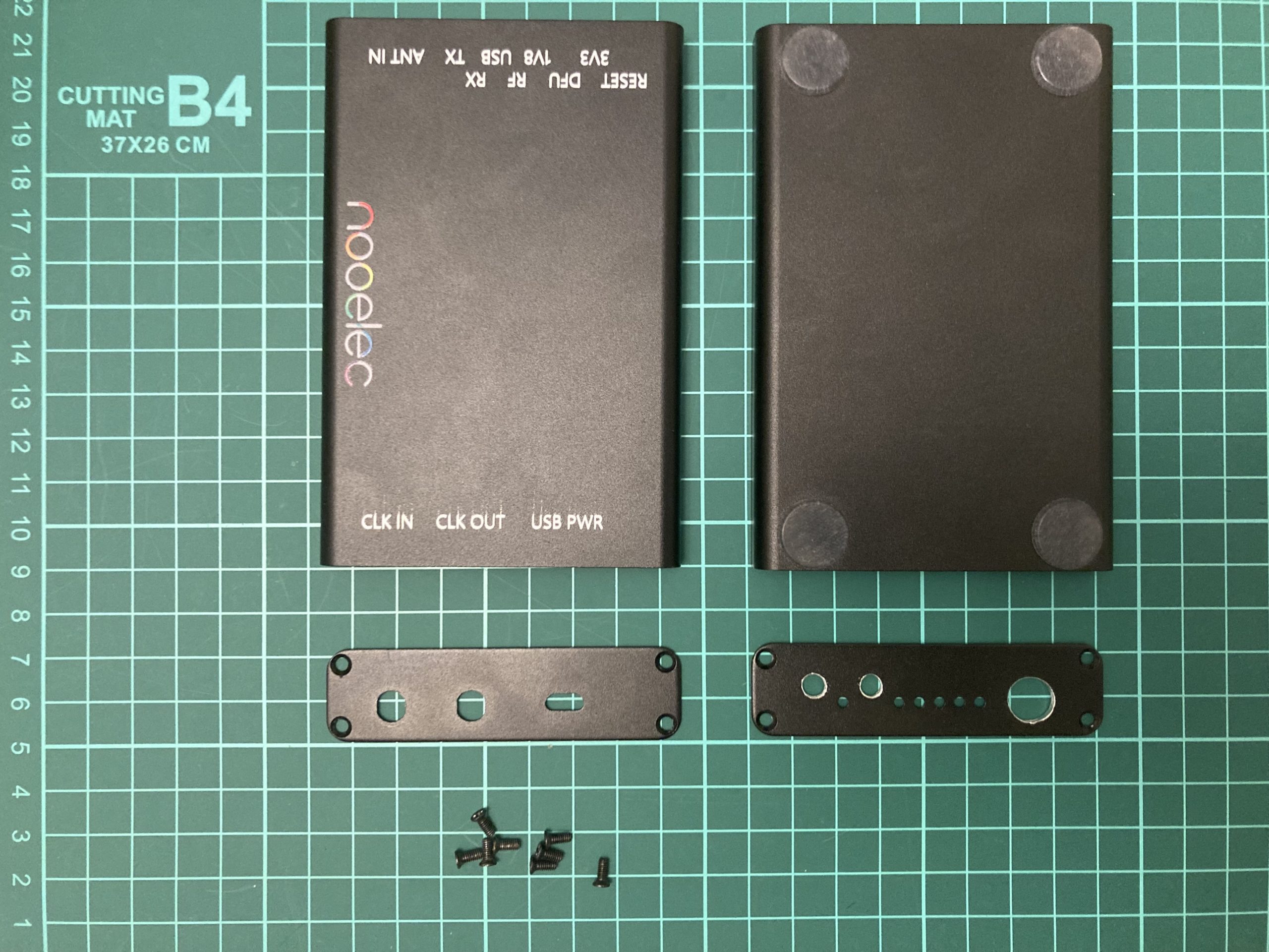
However, while installing the HackRF into the enclosure, we discovered that the enclosure’s length falls short by approximately 2-3 mm, preventing the case from closing completely. To address this problem, we needed to widen the existing holes by drilling, fortunately only from one side.

While this is not the optimal solution, it is certainly an improvement from the initial state. In total, we invested nearly $250 in the HackRF. This decision might not have been the wisest, considering we could have acquired the HackRF with the case and extra antennas for $100 less.
We are almost done except the … firmware. The case is that if you just remove the PortaPack and connect the HackRF with the PC, it won’t work. The reason is in software – remember I mentioned you have to switch the HackRF mode on to use it with the laptop? After removing the LCD display you are not able to do that. To fix that you need just to change the firmware from Portapack H2 Mayhem firmware onto the original HackRF one.
B. Antenna
The next item in our agenda is an antenna.
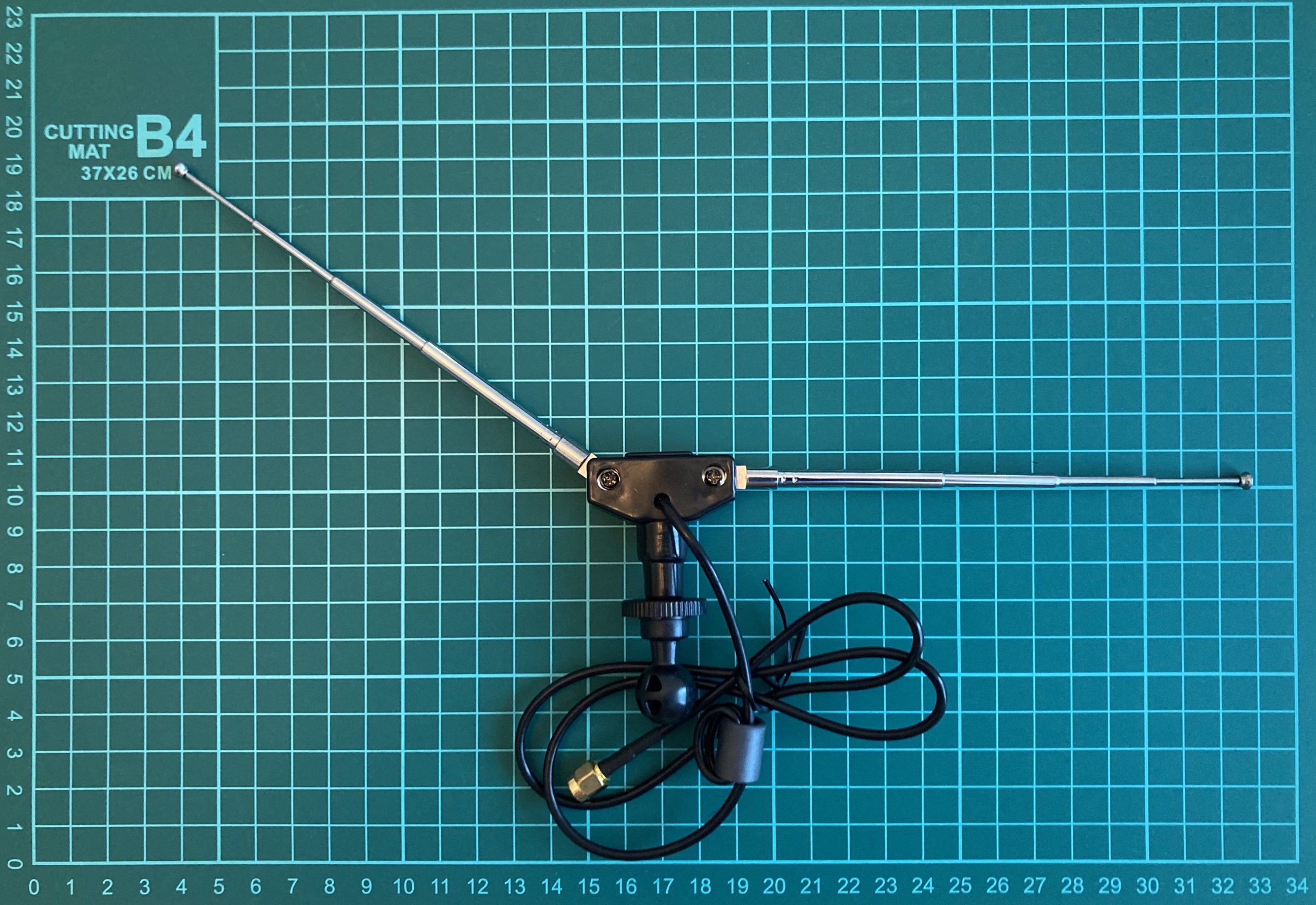
Our HackRF came with a basic telescopic antenna that served its purpose well in the initial stages. However, within a week or two of active usage, it became damaged.
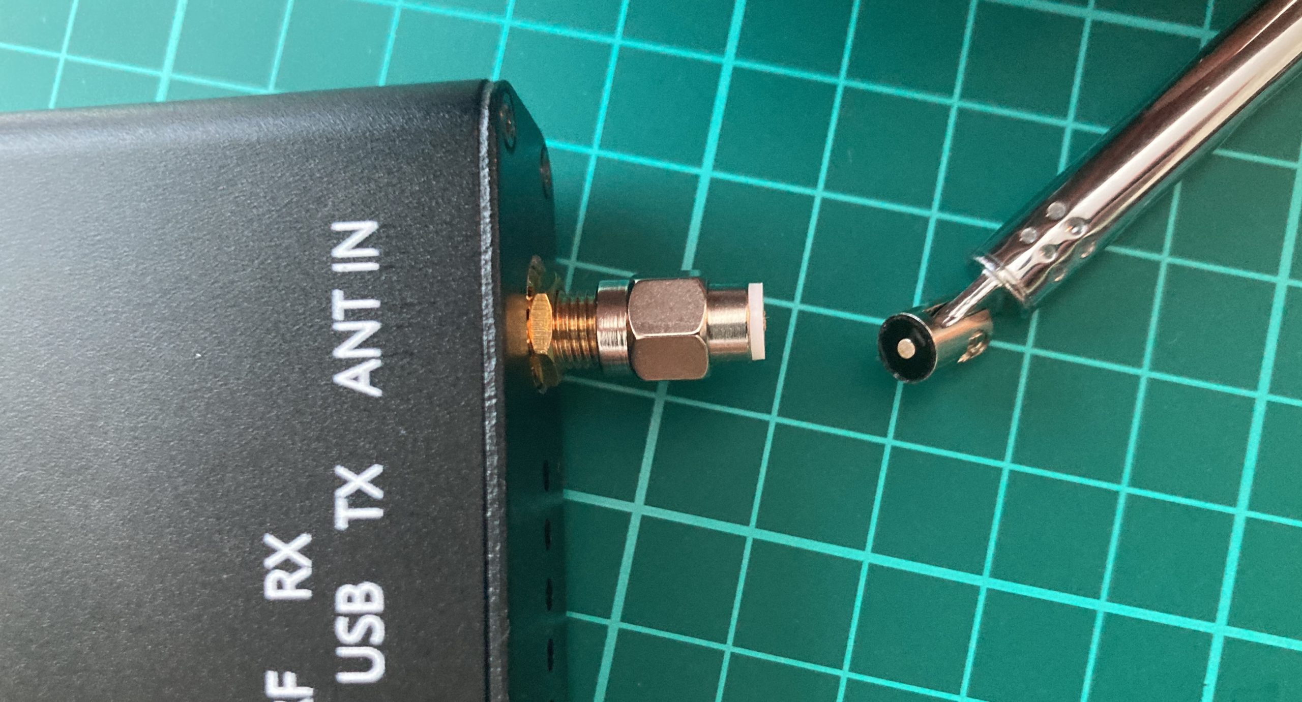
The slender 1.5 mm wide shaft unexpectedly fractured, echoing the disappointment we felt as we realized our activities were put on hold until we acquired a new antenna. While you might suggest using our Alfa Wi-Fi Adapter antenna and connecting it to HackRF, we’d like to explain why it’s not a straightforward solution. HackRF employs SMA ports for antenna connection.
However, here’s the twist: there are two varieties of SMA ports, namely SMA and RP-SMA. And to add another layer, each of these can have male and female connectors.
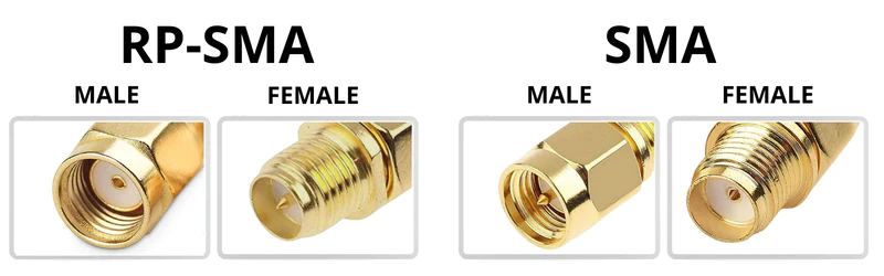
HackRF has the SMA Female connector hence the antenna has to be with SMA Male one (with a pin inside). Alfa has the RP-SMA Female connecter which means the antenna should be RP-SMA Male (without a pin inside).
Because the connectors differ, using the Alfa antenna with HackRF is not feasible. Although it may be physically possible to attach the Alfa antenna to the HackRF, the internal connectors are not compatible, rendering it ineffective.
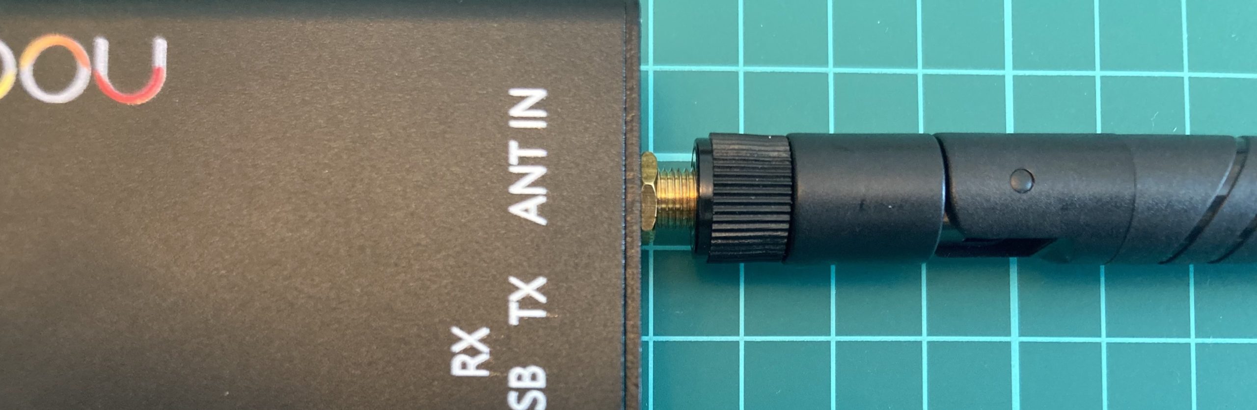
Disclaimer: due to our huge technical and life experience, we made that scheme work (HackRF with Alfa antenna) by putting staple pin inside the connector. But the link quality was not ideal and the connector could be broken so we highly recommend not to do that and to order the proper adapter or antenna.
Another reason why we took so much time talking about adapters is the money saving purchasing the equipment. Let’s compare 2 ads.
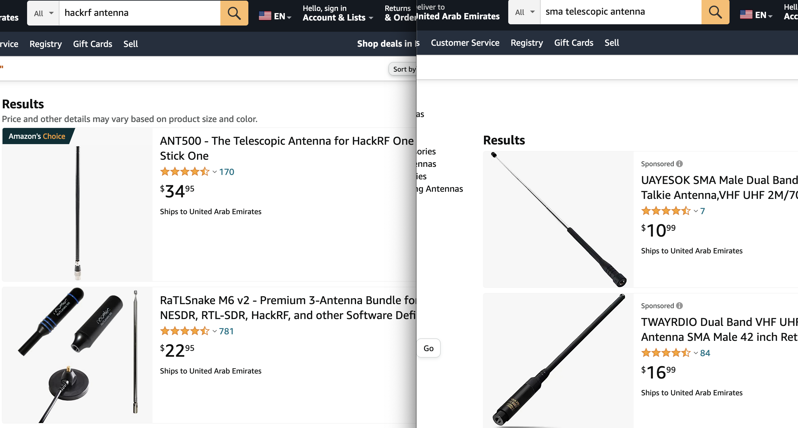
As you may see, the antennas are almost identical but the price difference is 2-3 times. Do you need additional expenses just for the “HackRF” name on the antenna? Moreover, as we think, it’s a market hook for lazy guys: if you don’t want to figure that out – please pay more for your lack of knowledge.
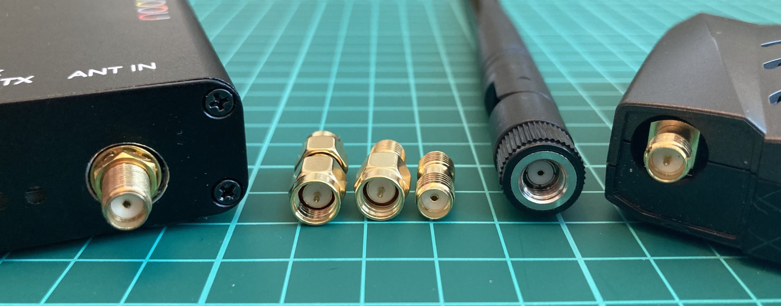
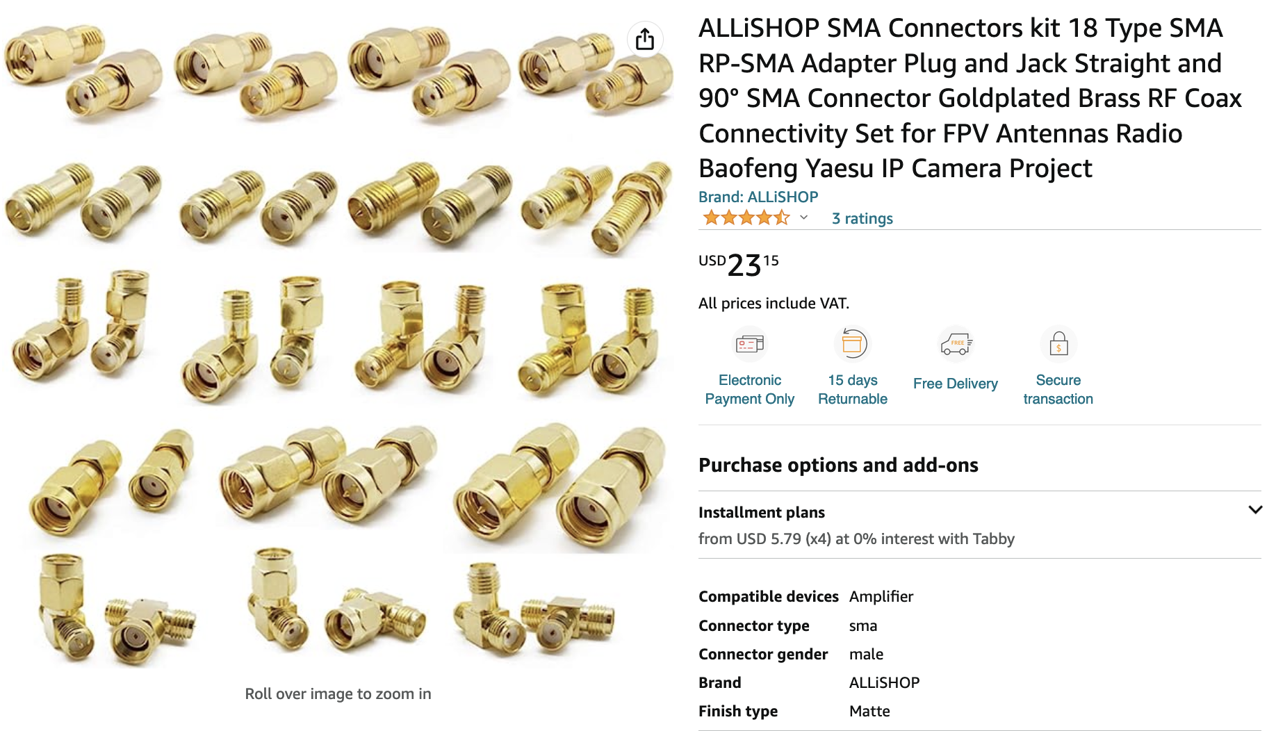
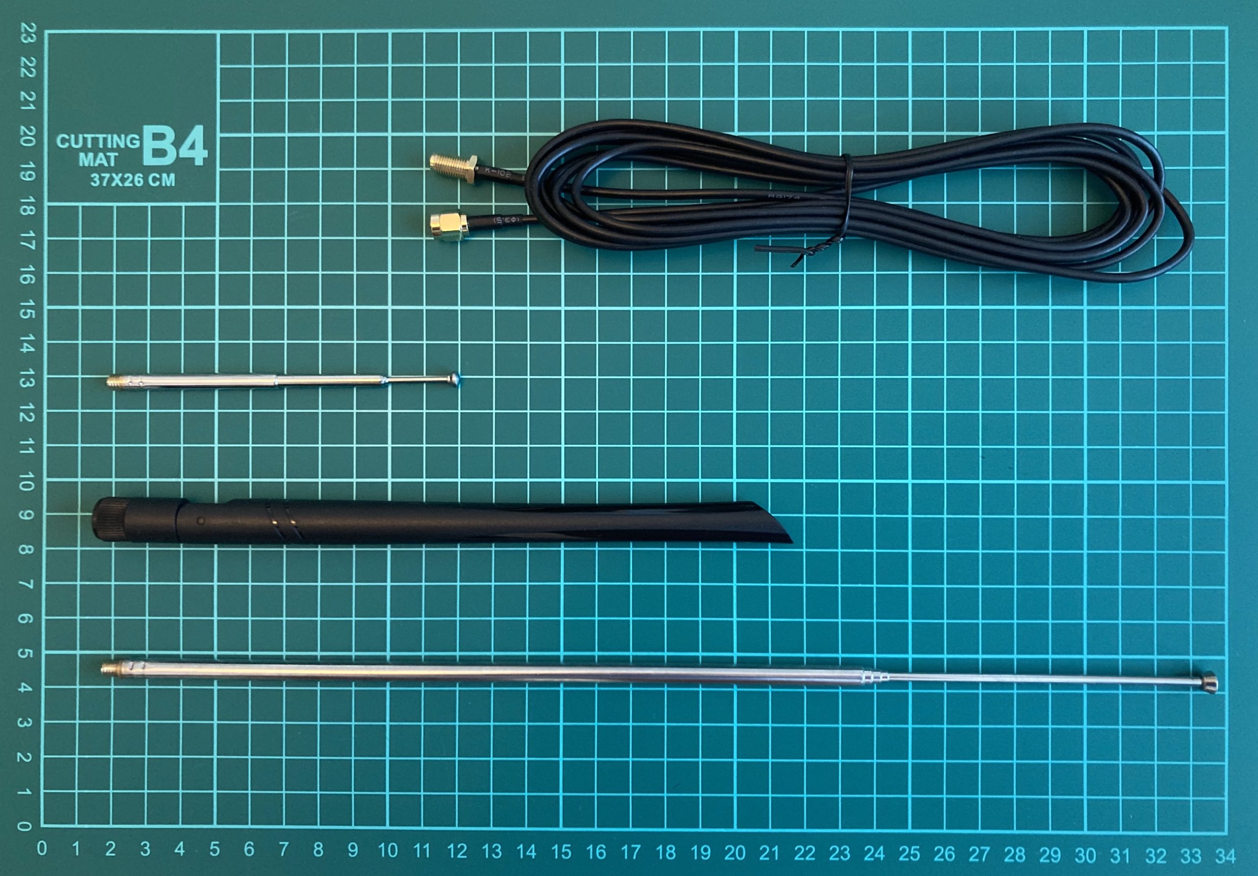
But we decided to go the other way. To solve the connector issue and to forget that like a scary dream, we purchased the adapter army for the all-possible situations.
Also, we learned the lesson with moving parts: to add flexibility, reliability and convenience of usage to the construction, we decided to go with a coaxial cable.
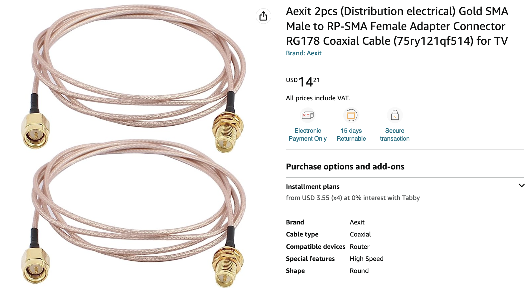
After all of the addons, using HackRF right now is like a driving a race car.
C. USB cable
The last important item we have to discuss about is a USB cable. It’s simply easy but there are several crucial points you have to keep in mind and follow to establish a connection at the first side and to make the signal strong and clear. First of all, not all of the USB cables have the ability to transfer the payload. Some of them are just using as a charger cable and vendors are making the manufacture cheap by excluding payload wires keeping only 5 volts transmitting. You can see 2 Micro USB – USB cables on the next picture which are almost identical. The difference is that the left one can transfer the data and the right one cannot.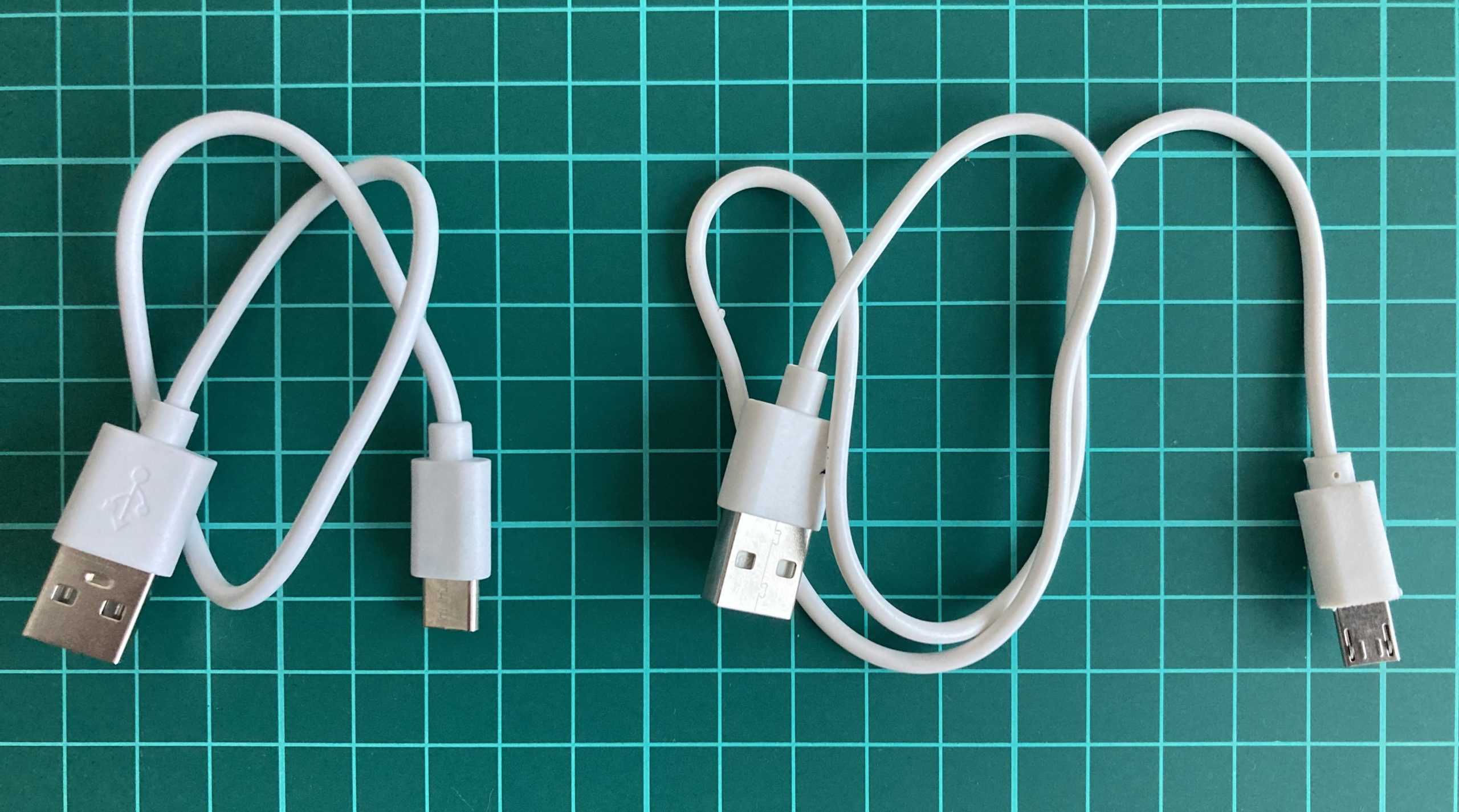
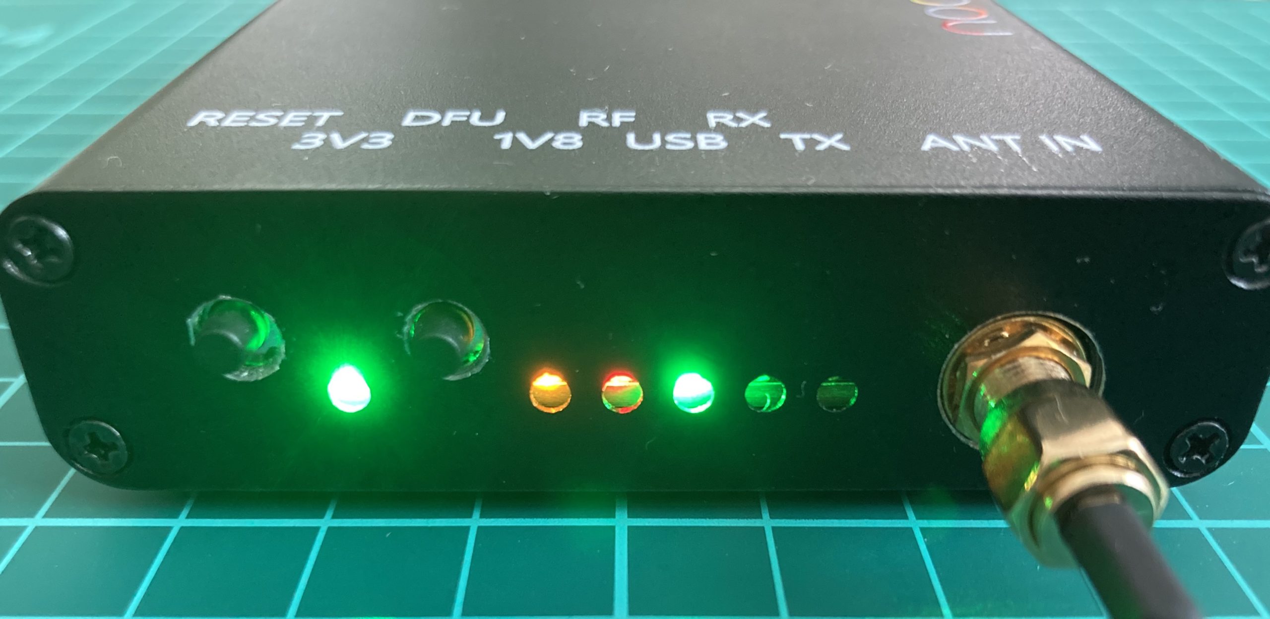
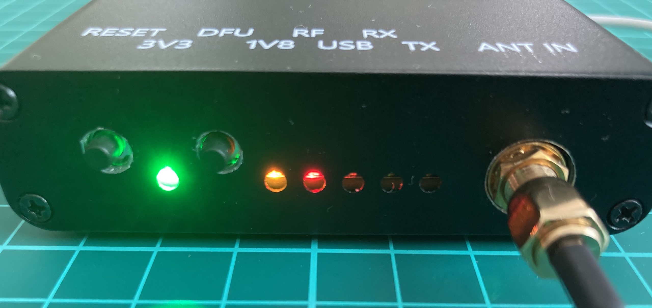
Let’s check that out by connecting both of them to the PC. The middle LED (green) is indicating that the HackRF is recognized as an USB device. As we can see on the left pictures the USB LED is on, on the right one – not.
Additionally, it’s crucial to utilize the shortest cable feasible. Opting for a cable longer than 180-200 cm could result in suboptimal results. With an increase in cable length, the expected signal loss also escalates. To illustrate, during the composition of this post, a 450 cm cable was tested, revealing that the HackRF device only powered up partially.
Furthermore, it is advisable to employ a USB cable that features shielding. The use of an unshielded cable heightens the potential for RF interference. To guarantee proper shielding, you can employ a continuity tester to validate that the shield on one connector maintains continuity with the shield on the connector situated at the opposite end of the cable.
Lastly, if feasible, opt for a cable equipped with a ferrite core. These cables are often marketed for their capacity to reduce noise and can be recognized by the inclusion of a plastic block situated towards one end.
2. Software
A. hackrf_
We would like to start with the default command-lines HackRF software which includes 8 native tools:
- hackrf_info
- hackrf_transfer
- hackrf_sweep
- hackrf_debug
- hackrf_clock
- hackrf_cpldjtag
- hackrf_operacake
- hackrf_spiflash
Operating through the command line means we can interact with HackRF by executing commands in a terminal or command prompt window. By leveraging HackRF capabilities, we can gain insights into wireless communication systems, experiment with different protocols, perform security research, and develop our own radio applications.
So, let’s consider all of them.
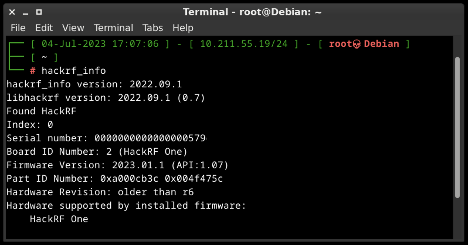
A.A. hackrf_info
The main purpose of hackrf_info is just to probe device and show configuration. That’s all, no additional keys or settings.
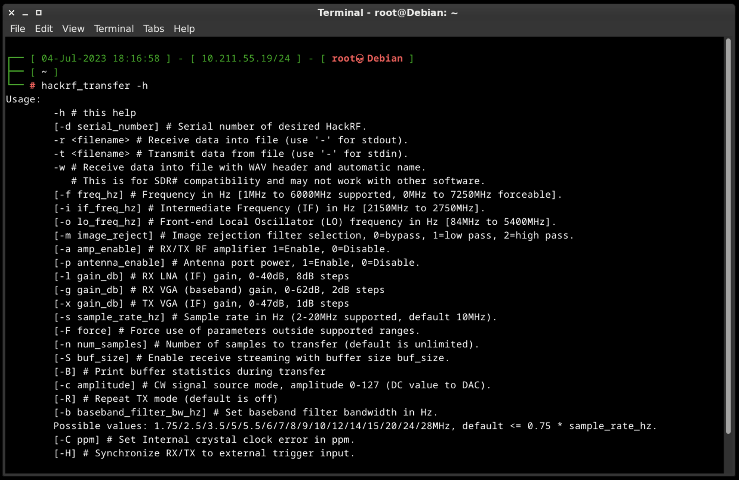
A.B. hackrf_transfer
This tool is specifically designed to capture or replay RF signals. It provides a convenient way to record radio signals from the air or play back recorded signals, enabling users to analyze and manipulate radio transmissions.
The tool allows us to specify parameters such as the frequency, sample rate, and gain settings for capturing or transmitting signals. We can save captured signals to a file for further analysis or use pre-recorded signals to simulate specific radio environments.
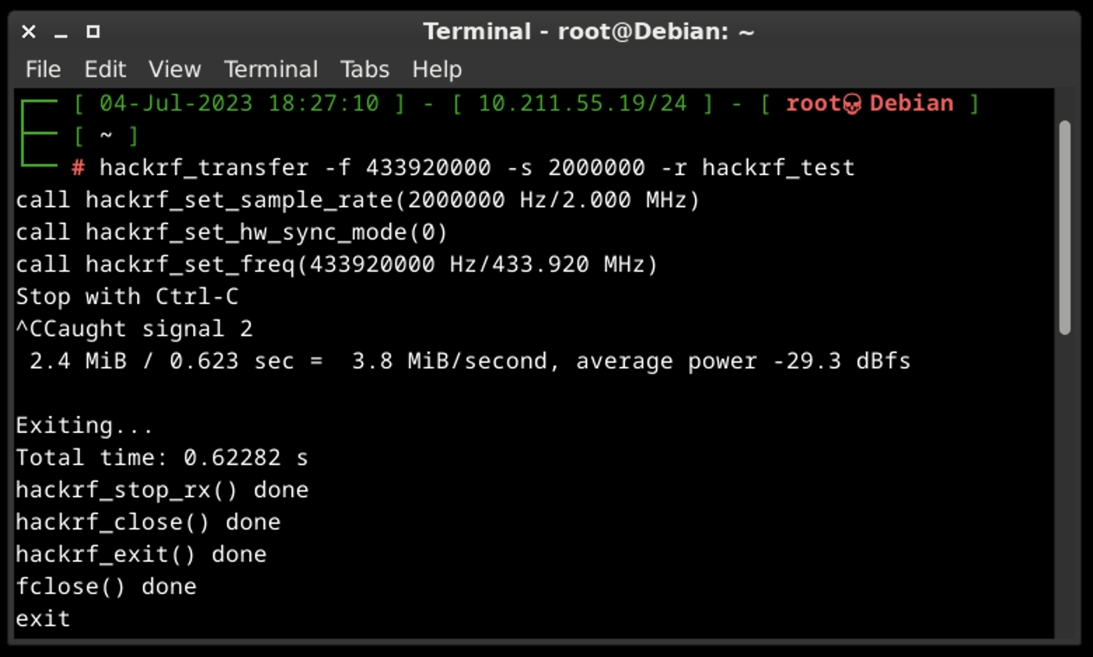
Some of the default commands:
- hackrf_transfer -f 433920000 -s 2000000 -r hackrf_test
This command means that we are receiving data into the file (-r key) on the 433,92 MHz frequency (-f key) with 2 MHz sample rate (-s key). For the main bunch of tests that command is more than enough.
- hackrf_transfer -f 433920000 -s 2000000 -t hackrf_test
This command means that we are transmitting data from the file (-t key) on the 433,92 MHz frequency (-f key) with 2 MHz sample rate (-s key). It’s a simple replay to the air what we saved previously.
A.C. hackrf_sweep
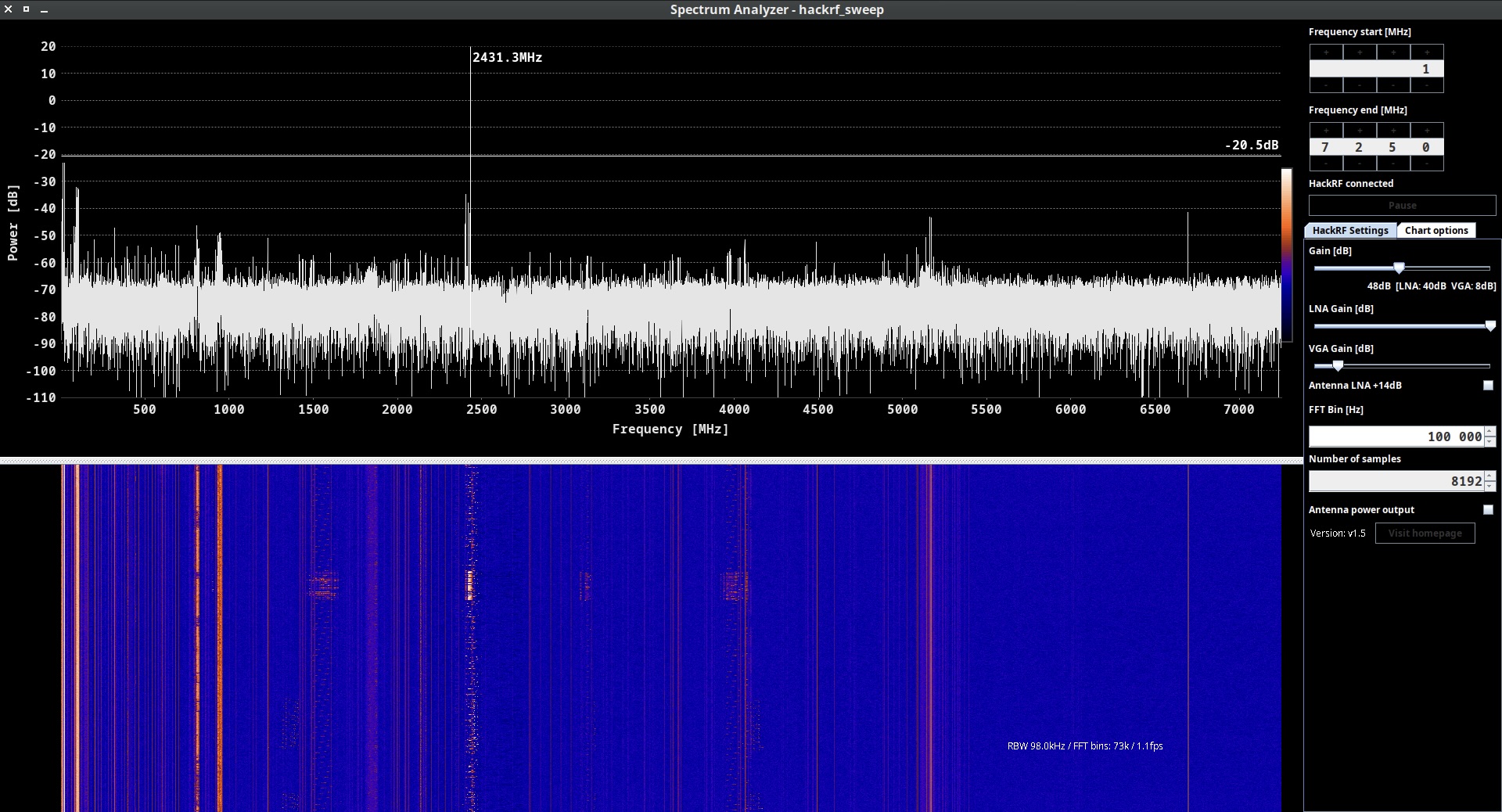
hackrf_sweep is a command-line spectrum analyzer – measurement instrument used to analyze and visualize the frequency components of a signal. It provides insights into the spectral characteristics of an input signal, showing how the signal’s power is distributed across different frequencies.
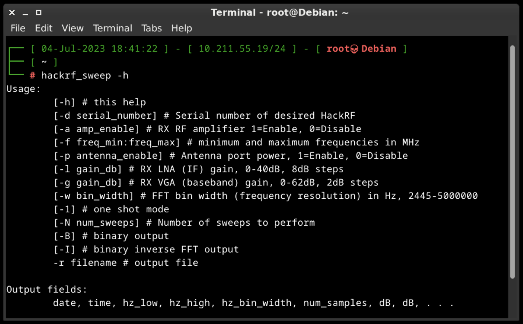
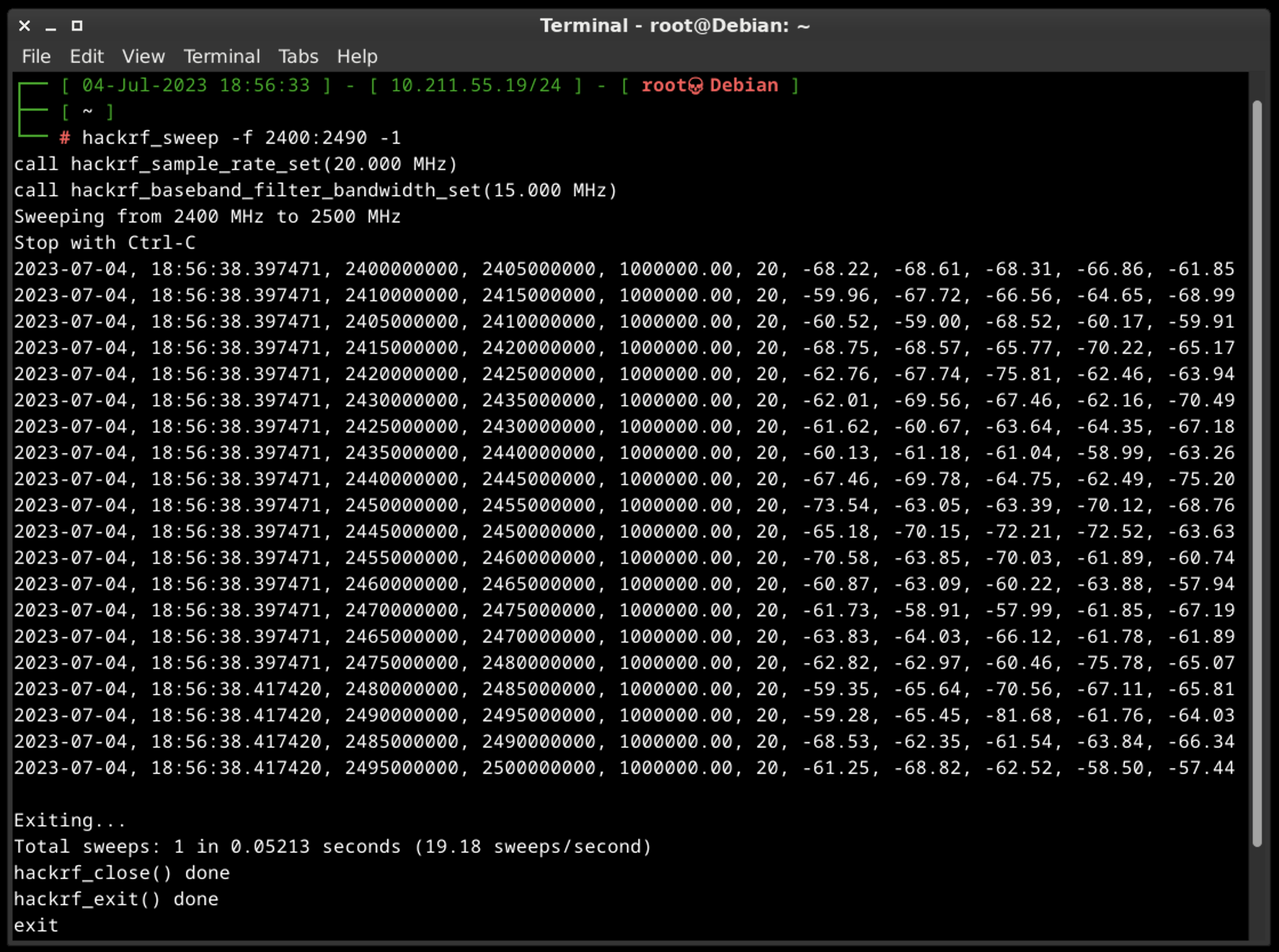
As the output we may see the date and time of the sweep (columns 1 and 2), low and high Hz sweep (columns 3 and 4), the width in Hz (1 MHz in this case) of each frequency bin (column 5), number of samples analyzed (column 6). Each of the remaining columns shows the power detected in each of several frequency bins. In this case there are five bins, the first from 2400 to 2405 MHz, the second from 2410 to 2415 MHz, and so forth.
We don’t think you will use hackrf_sweep in the wild as it is, but you definitely will use hackrf-spectrum-analyzer and/or QSpectrumAnalyzer as addons to it.
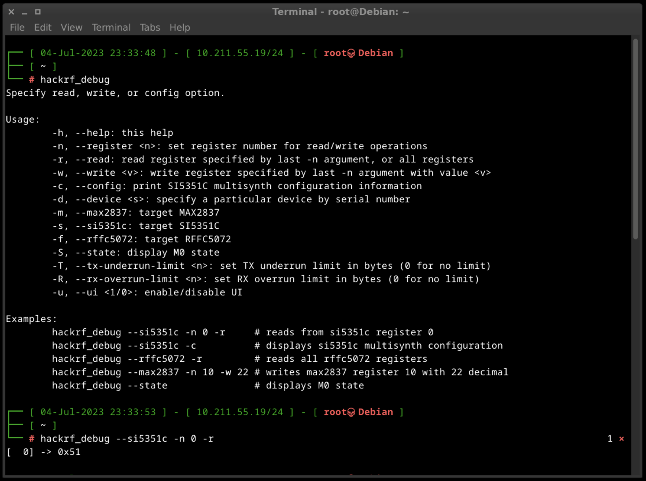
A.D. hackrf_debug
It is designed to assist with debugging and troubleshooting tasks (read and write registers and other low-level configuration). The tool provides various functionalities to aid in diagnosing issues and understanding the behavior of the HackRF. Some of the key features and capabilities of HackRF Debug include USB communication debugging, firmware logging and debug output.
It’s important to note that the app is primarily intended for advanced users, developers, and those involved in firmware or software development for the HackRF. If you’re experiencing issues with the HackRF or want to gain deeper insights into its operation, using hackrf_debug in conjunction with appropriate documentation and community support can be beneficial.
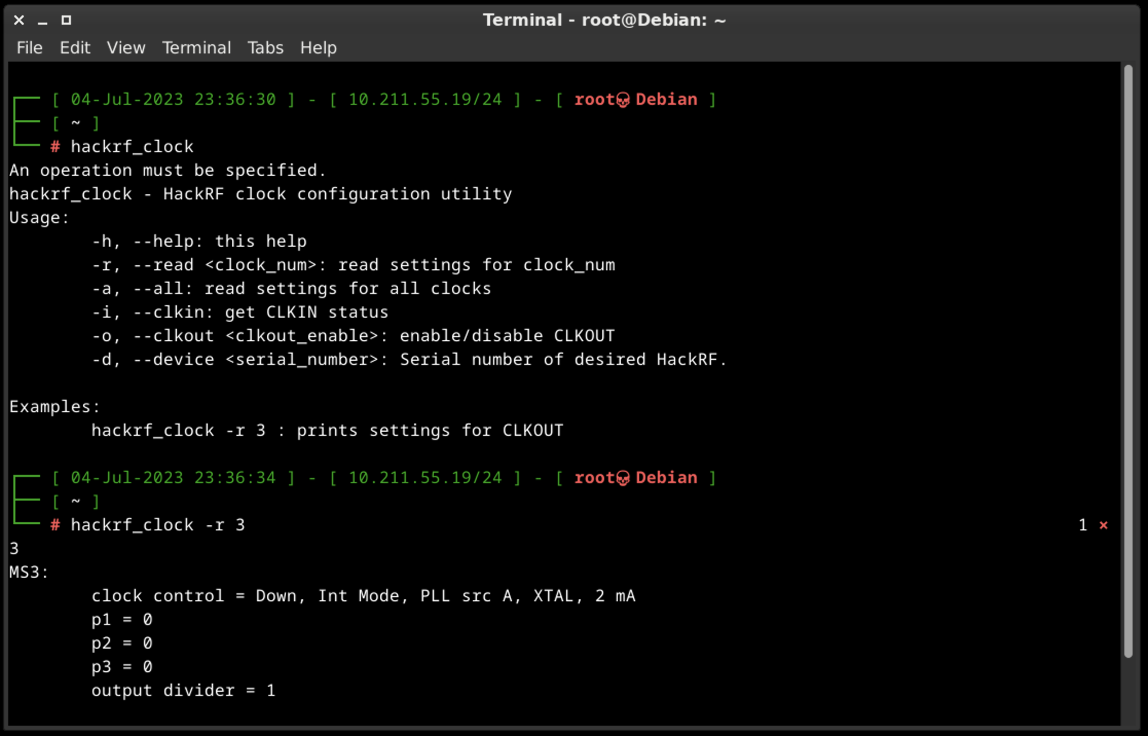
A.E. hackrf_clock
The HackRF One device incorporates a clock signal feature that operates at a frequency of 10 MHz. This clock signal is available on the CLKOUT port and is generated as a 3.3 V square wave. It is specifically designed to be compatible with high impedance loads.
The HackRF One also includes a CLKIN port, which serves as a high impedance input. It expects a 3.3 V square wave at a frequency of 10 MHz. It is crucial to ensure that the voltage does not exceed 3.3 V or drop below 0 V when using this input. Additionally, it is important to note that the CLKIN port only supports a clock signal at 10 MHz unless you modify the firmware to accommodate other frequencies. It is possible to directly connect the CLKOUT port of one HackRF One device to the CLKIN port of another.
When a clock signal is detected on the CLKIN port, the HackRF One switches from using its internal crystal to utilizing the external clock signal. This transition occurs when a transmit or receive operation begins.
To confirm whether a signal has been detected on the CLKIN port, you can use the hackrf_clock -i command. If a clock signal is detected, the expected output will be “CLKIN status: clock signal detected.” If no clock signal is detected, the expected output will be “CLKIN status: no clock signal detected.” This command allows you to verify the presence or absence of a clock signal on the CLKIN port.
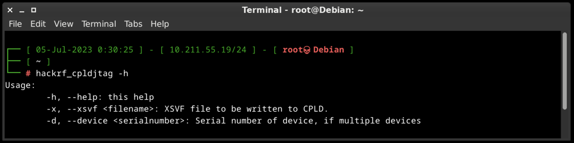
A.F. hackrf_cpldjtag
The main idea of hackrf_cpldjtag is to perform programing CPLD.
In the context of HackRF, the term “CPLD” refers to the Complex Programmable Logic Device and using to handle various functions and interactions within the device.
The CPLD is responsible for managing tasks such as controlling the USB interface, handling data transfers between the host computer and the HackRF hardware, and coordinating the functionality of different components within the device.
By utilizing the capabilities of the CPLD, it’s allowing users to transmit and receive a wide range of radio frequencies, perform spectrum analysis, and experiment with various wireless communication protocols.
The specific functions and programming of the CPLD in HackRF are integral to the device’s operation but are typically managed internally by the firmware and software libraries. As an end-user, you may not directly interact with or program the CPLD, but you can take advantage of its capabilities through the supported software and firmware provided by the HackRF community.
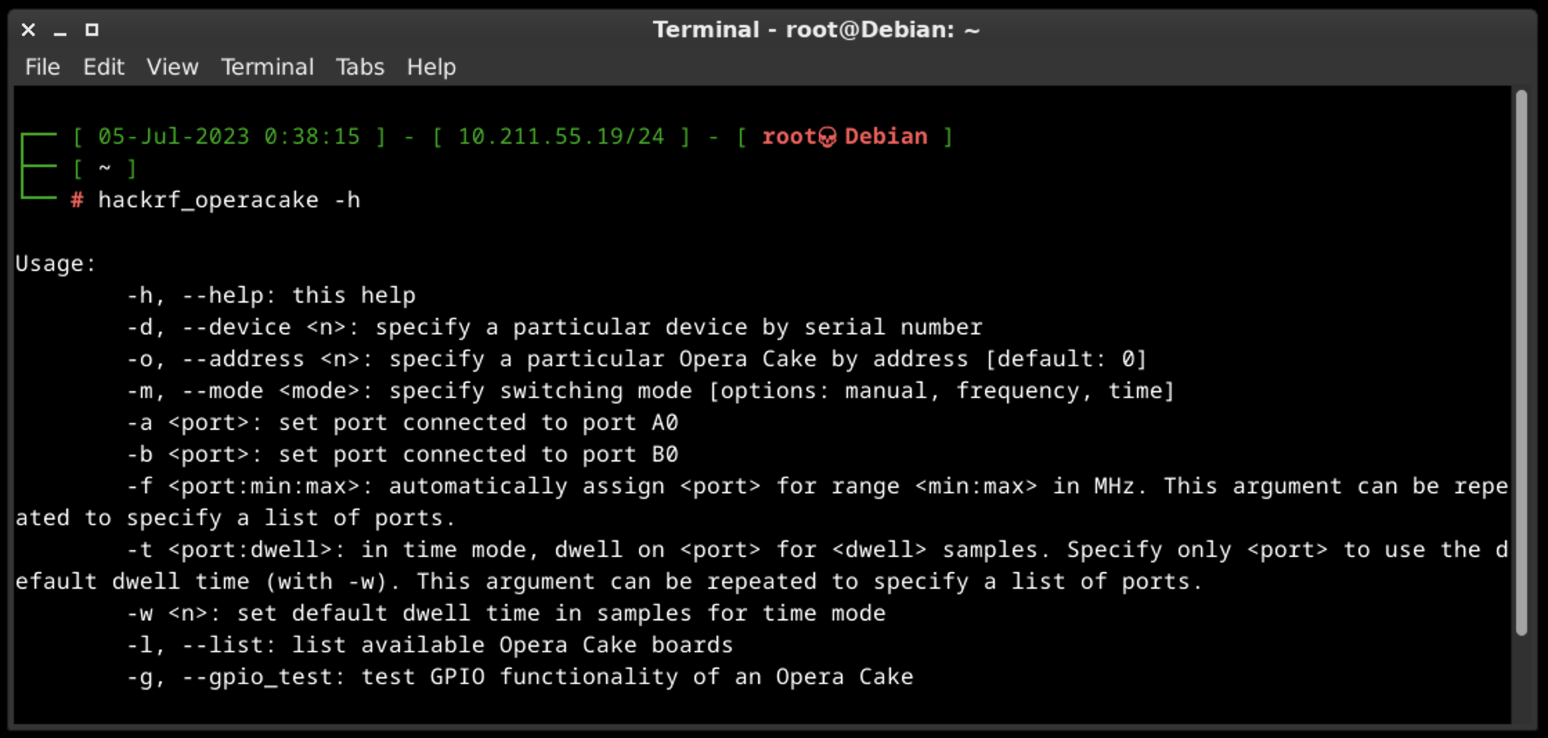
A.G. hackrf_operacake
Opera Cake is an add-on board designed for HackRF that enables antenna switching capabilities. It consists of two 1×4 switches and includes a cross-over switch that allows it to function as a 1×8 switch. Multiple Opera Cake boards can be stacked onto a single HackRF, as long as each Opera Cake has a unique board address assigned to it.
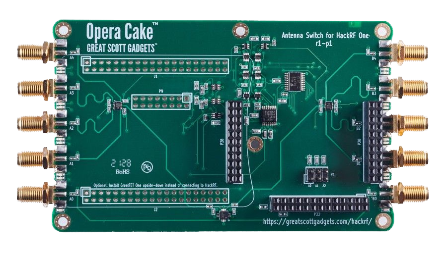
By using Opera Cake as a 1×8 switch, you can connect multiple antennas to your HackRF One simultaneously. This allows you to switch between different antennas in software without physically swapping the hardware connections. For example, you can connect a long wire antenna for HF bands, a discone antenna for VHF and UHF, a dipole antenna for 2.4 GHz, and a dish antenna for satellite bands. The software control provided by Opera Cake simplifies the antenna selection process.
Alternatively, when configured as a pair of 1×4 switches, Opera Cake can be used as a switched filter bank. By connecting specific ports of the switches (A1 to B1, A2 to B2, A3 to B3, A4 to B4) with SMA filters and cables of your choice, you can easily switch between different filters for your transmit or receive operations. This eliminates the need to physically reconnect hardware each time you want to use a different filter.
To configure and control Opera Cake, you can utilize the hackrf_operacake command-line tool which allows you to set up the desired switching configurations and manage the operation.
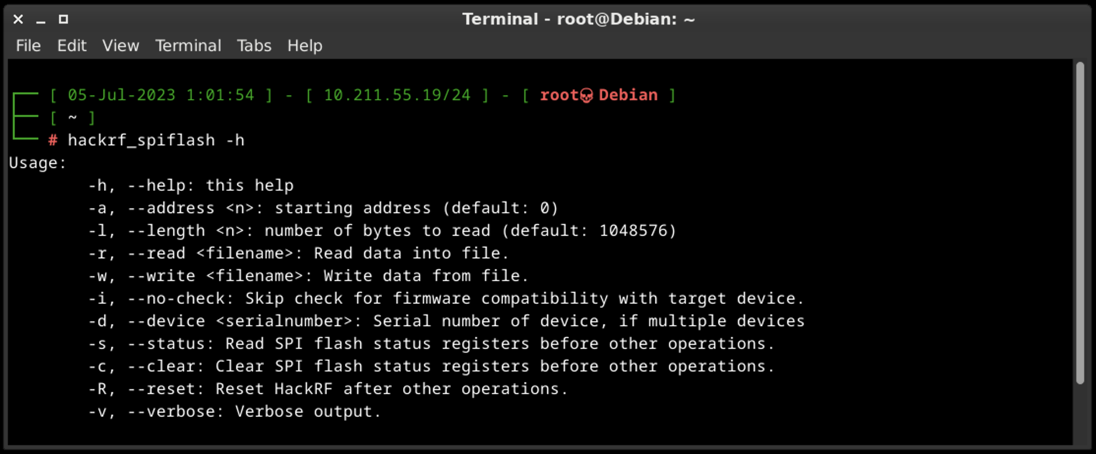
A.H. hackrf_spiflash
hackrf_spiflash is used for reading from, writing to, and erasing the SPI flash memory that is present on the HackRF board.
The SPI flash memory stores the firmware and configuration settings of the device. It allows for the persistent storage of firmware updates, custom settings, and other data related to the operation of the HackRF.
The hackrf_spiflash tool provides commands to interact with the SPI flash memory. Here are some of the key functionalities it offers:
- Reading: You can use hackrf_spiflash to read the content of the SPI flash memory. This allows you to retrieve the firmware or configuration data stored on the flash memory.
- Writing: The tool enables you to write data to specific regions of the SPI flash memory. This is useful for updating the firmware or configuring custom settings on the HackRF One.
- Erasing: Hackrf_spiflash supports erasing specific sectors or the entire SPI flash memory. This operation is often required before writing new data to the flash memory.
It’s important to exercise caution when using the hackrf_spiflash tool because improper usage or incorrect data manipulation can result in firmware corruption or loss of functionality in the HackRF device.
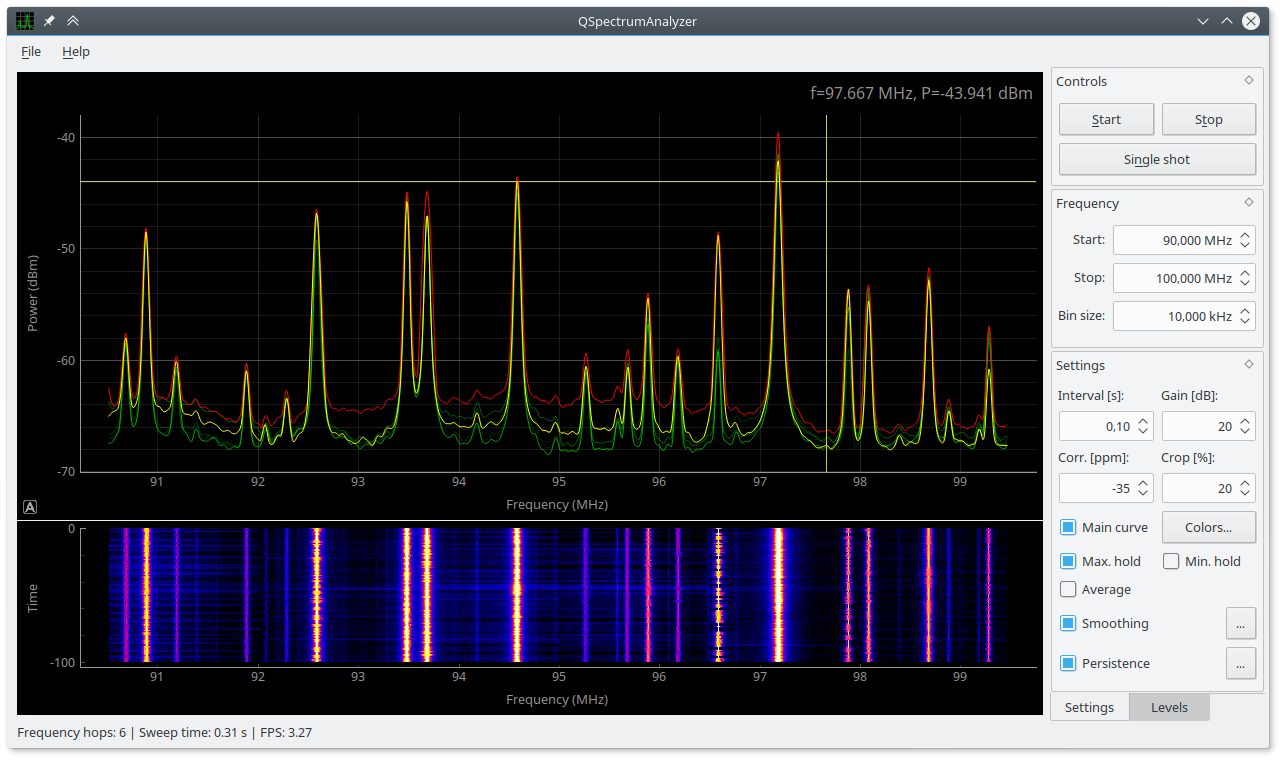
B. QSpectrumAnalyzer and hackrf_spectrum_analyzer
Spectrum analyzers allow us to analyze RF signals in terms of their frequency, amplitude, and power levels. By examining the frequency spectrum, we can identify the presence of signals, measure their strength, and determine characteristics such as modulation types, bandwidth, and harmonics.
Also, spectrum analyzers are valuable tools for troubleshooting RF systems. They enable to identify and locate issues such as unwanted spurious emissions, noise sources, and signal distortions. By analyzing the spectrum, they can pinpoint problematic frequencies, assess signal quality, and make adjustments to improve system performance.
The last, but not least, spectrum analyzers are extensively used in research and development of wireless technologies, such as wireless communication protocols, radar systems, IoT devices, and electronic instrumentation.
QSpectrumAnalyzer and hackrf_spectrum_analyzer are two tools used for spectrum analysis. They are quite similar and have the same features so it’s depends on you which tool is using.
C. SDRSharp aka SDR# / CubicSDR / GQRX
All of the highlighted tools are popular software applications used for SDR reception and signal processing. They provide a user-friendly interface for interacting with HackRF and other SDR hardware and analyzing RF signals. Here’s an overview of each application:
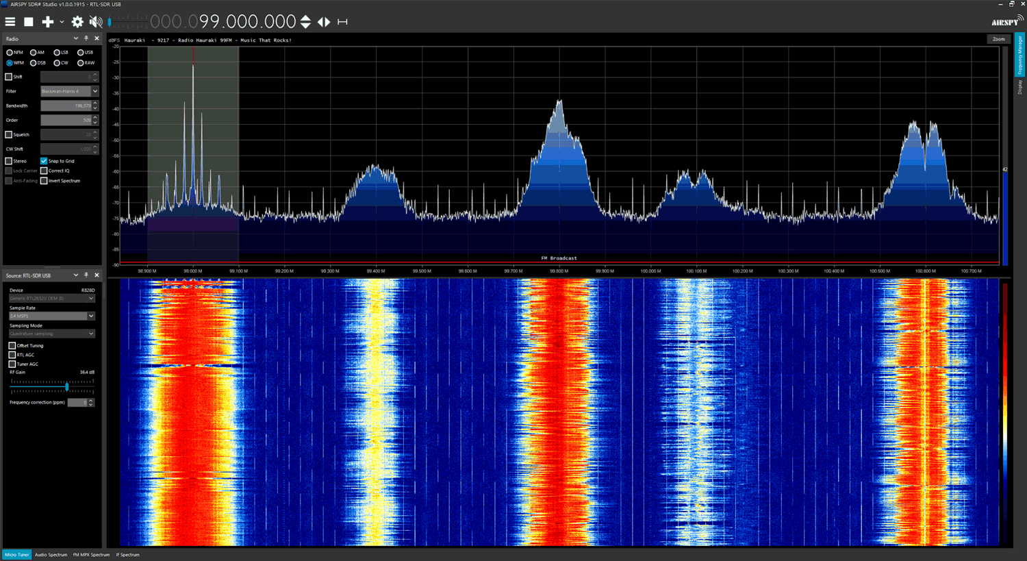
C.A. SDRSharp (SDR#)
SDRSharp, often referred to as SDR#, is a widely used SDR application for Windows. It supports a variety of SDR devices and allows users to tune into different frequency bands, visualize RF signals, and demodulate various modulation types. SDR# offers a customizable and intuitive user interface with features like spectrum display, waterfall plot, signal recording, and audio playback. It also supports plugins, enabling users to extend its functionality.
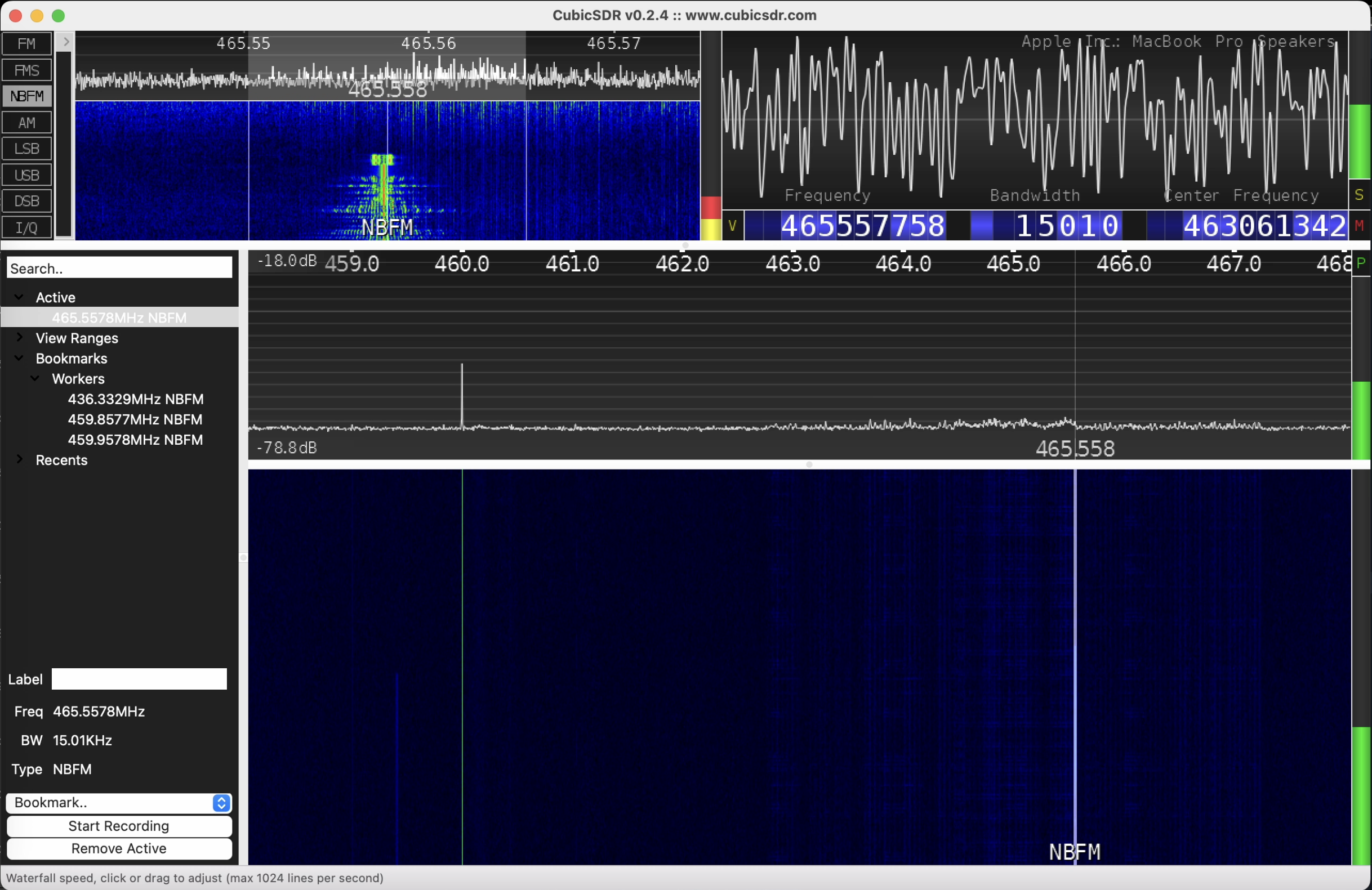
C.B. CubicSDR
CubicSDR application available for multiple platforms, including Windows, macOS, and Linux. It provides a 3D visualization of the RF spectrum, offering a panoramic view of the signals. CubicSDR supports various SDR hardware devices and allows users to tune into frequencies, adjust bandwidth, apply filters, and demodulate signals. It also offers features such as signal recording, playback, and remote network operation.
We will work closely with it further.
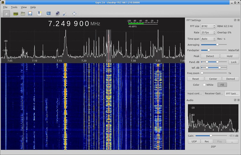
C.C. GQRX
Remembering the app’s name on the first try can be challenging, especially if you’re unaware of its background.
The name “GQRX” is derived from the combination of three parts:
- “G” stands for GNU: GQRX is part of the GNU Radio project, which is a free and open-source software toolkit for building and exploring radio communication systems
- “Q” represents the Qt C++ toolkit: GQRX is built using the Qt framework, which is a popular C++ library for creating cross-platform applications with a graphical user interface (GUI)
- “RX” represents the reception of signals. The name GQRX emphasizes its role as a radio receiver application.
GQRX is designed primarily for Linux-based systems, although it is also available for macOS and Windows. It supports a wide range of SDR hardware devices and provides a user-friendly interface for signal reception and analysis. GQRX offers real-time spectrum visualization, signal demodulation, and audio output. It supports various demodulation modes, including AM, FM, SSB, CW, and digital modes like ADS-B and APRS and supports plugins for extended functionality.
Main Differences:
- Platform: SDRSharp is primarily designed for Windows, while CubicSDR and GQRX are available for multiple platforms, including Windows, macOS, and Linux.
- User Interface: SDRSharp provides a customizable interface with spectrum and waterfall displays, while CubicSDR offers a unique 3D spectrum visualization. GQRX provides a user-friendly interface with real-time spectrum display.
- Features: All three applications offer basic functionalities like frequency tuning, demodulation, and spectrum visualization. However, the availability of advanced features and plugins may vary between the applications.
It’s important to note that these applications continue to evolve with new features and improvements, so it’s recommended to check their respective websites for the latest information and updates.
D. SDRAngel
SDRAngel is an open-source software application designed for SDR purposes. It provides a flexible and feature-rich environment for receiving, processing, and transmitting RF signals. SDRAngel is compatible with various SDR hardware devices including HackRF and can be used on different operating systems, including Windows, macOS, and Linux.
Here are some key features and capabilities of SDRAngel:
- Receiver and Spectrum Analyzer: SDRAngel offers a wide range of receiver options, including AM, FM, SSB, CW, digital modes (such as DMR, D-Star, P25, and more), as well as custom demodulation using GNU Radio flowgraphs. It provides a spectrum analyzer for real-time visualization of RF signals with adjustable settings like frequency range, span, and resolution bandwidth.
- Transmitter: SDRAngel allows to transmit signals using HackRF. It supports various modulation types and provides options for adjusting parameters like frequency, gain, and sample rate. The ability to transmit signals makes SDRAngel suitable for applications such as amateur radio experimentation and digital voice modes.
- Digital Signal Processing (DSP): SDRAngel includes a range of digital signal processing features, including filters, equalizers, decimators, and more. These DSP tools enable users to process received signals, improve signal quality, and remove unwanted noise or interference.
- Remote Network Operation: SDRAngel supports remote network operation, which means that the software can be used to control and interact with SDR hardware located on a different machine or network. This feature is useful for setting up distributed SDR systems or remotely accessing SDR devices.
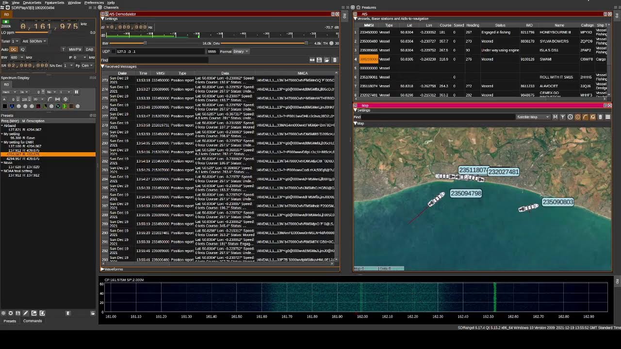
- Plugin Support: SDRAngel supports plugins, allowing users to extend its functionality. Plugins can be developed using the provided API and SDK, enabling customization and the addition of new features to suit specific requirements.
SDRAngel has gained popularity among SDR enthusiasts, researchers and hackers due to its extensive features, compatibility with various SDR devices, and open-source nature, which encourages community involvement and continuous development. It provides a powerful platform for exploring and experimenting with different aspects of software-defined radio.
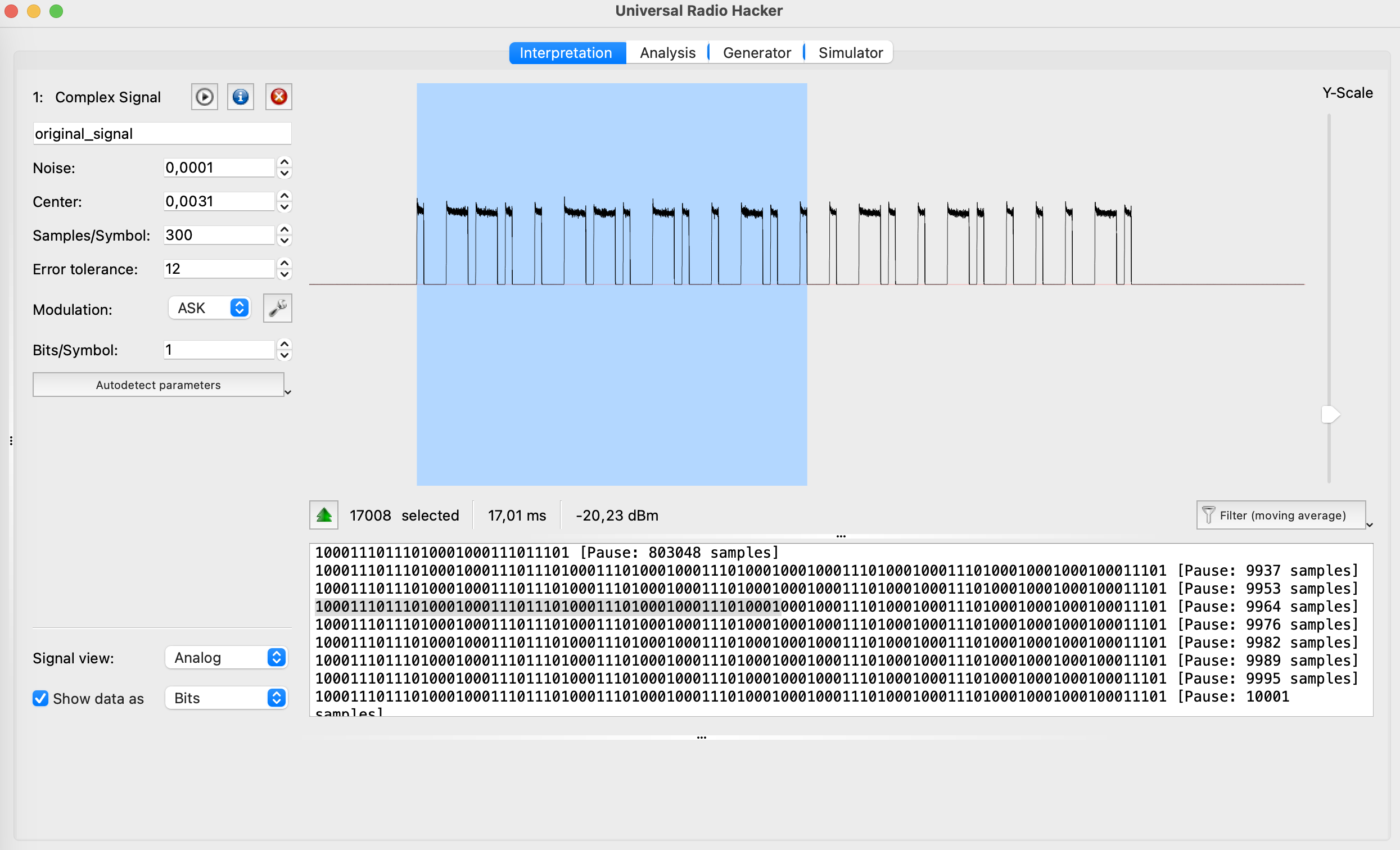
E. Universal Radio Hacker
Universal Radio Hacker (URH) is an open-source software tool designed for analyzing and reverse engineering various wireless communication protocols. It provides a user-friendly graphical interface and a set of features that enable users to capture, demodulate, decode, and analyze wireless signals.
Key features of Universal Radio Hacker include:
- URH allows users to capture radio signals from various SDR hardware devices like HackRF and import pre-recorded signal files. It provides a spectrum analyzer for visualizing the captured signals and offers options for adjusting frequency range, span, and resolution bandwidth.
- URH supports a wide range of modulation schemes, including amplitude modulation (AM), frequency modulation (FM), phase-shift keying (PSK), quadrature amplitude modulation (QAM), and more. It provides demodulation capabilities to recover the baseband signal from the captured RF signal. URH also offers decoding capabilities for many common wireless protocols, such as Bluetooth, Zigbee, RFID, and wireless key fobs.
- URH enables users to analyze and reverse engineer wireless protocols. It provides tools to identify packet boundaries, extract and display protocol fields, and perform protocol-specific analysis. Users can define custom protocol decoders and specify field definitions to decode and interpret captured packets.
- URH allows users to inject or replay captured or custom-generated packets into the wireless communication system. This feature is useful for testing and simulating scenarios, as well as for analyzing the behavior of the target system under different packet sequences.
- URH provides tools for manipulating captured signals, such as filtering, amplifying, and resampling. It also allows users to generate custom signals and modulate them for transmission. This capability is valuable for testing and experimentation purposes.
- URH has an active community of users and developers who contribute to the project. The software supports plugins, allowing users to extend its functionality or create custom decoders for specific wireless protocols. This extensibility enhances the versatility and adaptability of URH.
Universal Radio Hacker is a versatile tool that can be used for security research, protocol analysis, and wireless system testing. With its user-friendly interface and comprehensive range of features, the software becomes accessible to individuals new to the field as well as those with extensive experience in wireless communication analysis and reverse engineering.
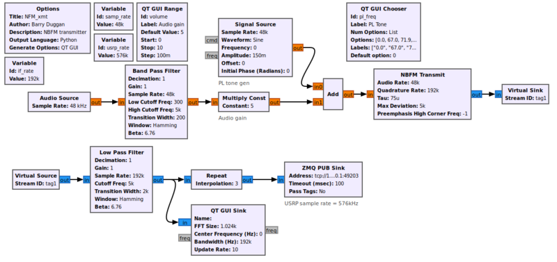
F. GNU Radio Companion
GNU Radio is an open-source software development toolkit widely used for the implementation of SDR systems. It provides a framework and a collection of signal processing blocks that enable the creation of radio systems for various applications. GNU Radio is designed to be flexible, modular, and customizable, allowing users to build complex SDR applications with ease.
Let’s consider its main keys:
- GNU Radio provides a vast library of signal processing blocks that perform operations such as filtering, modulation, demodulation, decoding, encoding, and more. These blocks can be connected together in a flowgraph to create a complete signal processing chain. GNU Radio offers both basic building blocks and advanced blocks for various communication protocols and modulation schemes.
- The primary design paradigm in GNU Radio is a flowgraph, which is a graphical representation of signal processing blocks connected together to form a data flow path. The flowgraph approach allows users to visually design and modify signal processing chains, making it easier to understand and implement complex SDR systems.
- Provides a hardware abstraction layer (HAL) that enables the use of a wide range of SDR hardware devices from different manufacturers. This abstraction layer allows users to interface with various SDR platforms, such as USRP, HackRF, LimeSDR, RTL-SDR, and more, without having to deal with the low-level hardware details.
- Support for Multiple Programming Languages: GNU Radio is primarily implemented in C++ and Python, offering flexibility and ease of use. Users can develop signal processing blocks and applications using either of these languages, allowing for rapid prototyping and development. The Python bindings in GNU Radio provide a high-level interface, making it accessible to a wide range of users, including those without extensive programming experience.
- It is highly extensible, allowing users to develop their own signal processing blocks and contribute them to the community. This extensibility enables the customization and expansion of GNU Radio’s functionality to suit specific requirements or to support new communication standards.
- It has a vibrant and active community of users and developers who collaborate, share knowledge, and contribute to the project. The community provides support, documentation, tutorials, and numerous ready-to-use examples and projects that help newcomers and experienced users alike.
GNU Radio is widely used in various domains, including wireless communication, defense, aerospace, research, education, and hobbyist projects. It provides a powerful and flexible platform for developing and experimenting with SDR systems and is an essential tool in the software-defined radio ecosystem.
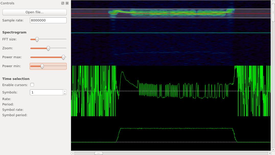
G. Inspectrum
Inspectrum is a DSP software tool used for analyzing and visualizing RF signals. It is designed for various applications, including wireless communication protocols, radio broadcasting, spectrum monitoring, and signal analysis.
Inspectrum provides a user-friendly interface that allows users to import RF signal data captured from various sources, such as SDRs or other RF signal receivers. Once the signal data is loaded into the software, Inspectrum offers a range of tools and features to explore and analyze the signal.
One of the key functionalities of Inspectrum is its ability to display and visualize the spectrum of a signal. It provides a real-time spectrogram that shows the power levels of different frequencies over time, allowing users to identify frequency components, modulation schemes, and other signal characteristics.
Inspectrum also supports demodulation and decoding of common RF protocols, making it useful for reverse engineering and analyzing wireless communication systems. It can automatically detect and decode signals using built-in decoders for popular protocols like AM, FM, SSB, Bluetooth, Wi-Fi, and many others. Additionally, users can create custom decoders for proprietary or less common protocols.
The software offers various analysis tools and features to help users understand the properties and behavior of RF signals. These include the ability to zoom in and out on specific parts of the signal, measure power levels and frequency deviations, apply filters and signal processing techniques, and export data for further analysis or documentation.
Inspectrum, an open-source initiative, can be accessed across various operating systems such as Windows, macOS, and Linux. Its inclusive approach enables the community to actively participate in its enhancement, introducing fresh features and refining its capabilities progressively.
Overall, Inspectrum is a powerful tool for RF signal analysis and exploration, providing users with the means to visualize, decode, and understand RF signals in a wide range of applications.
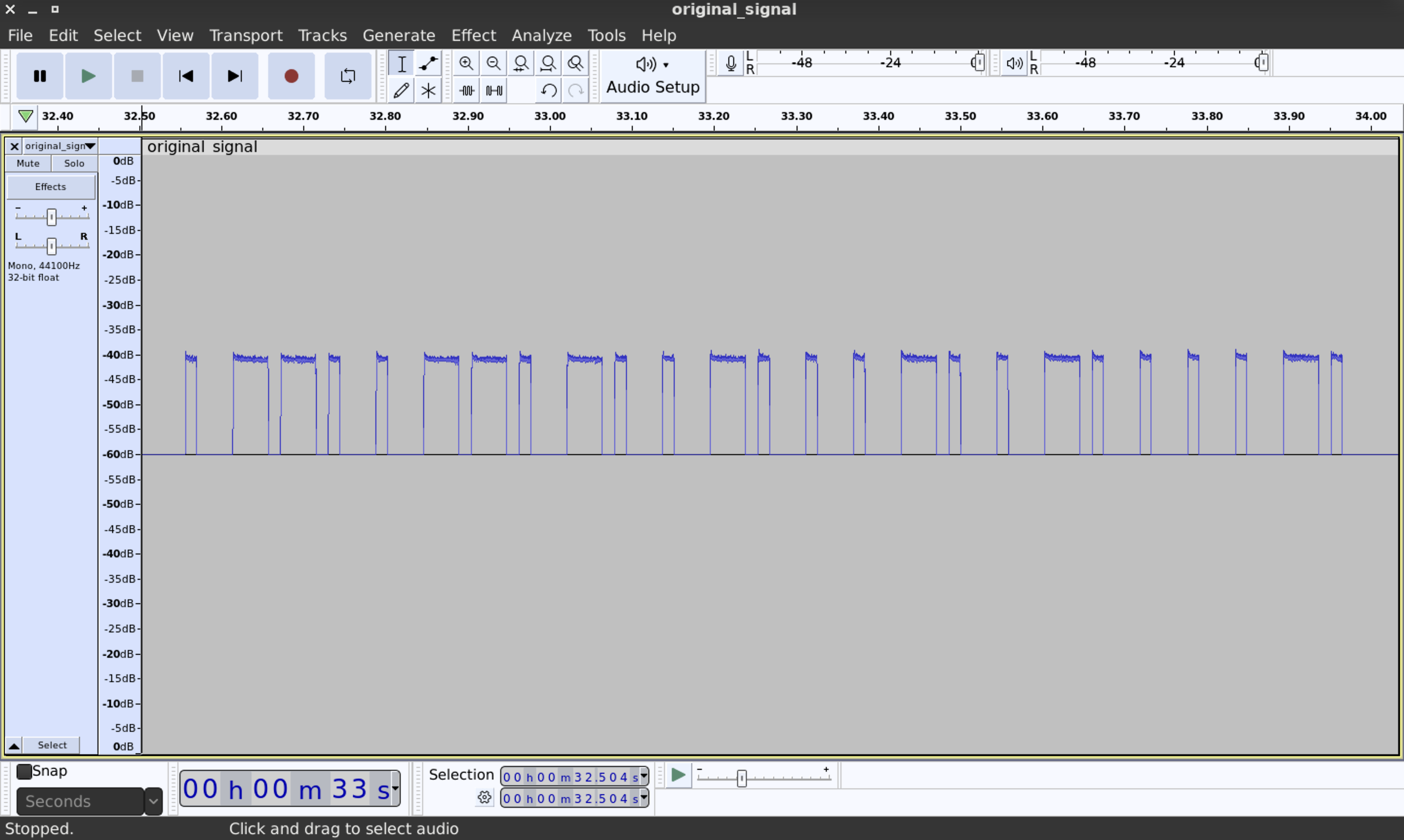
H. Audacity
While Audacity is primarily known as an audio editing and recording software, it can also be utilized in conjunction with SDRs for certain applications.
Here’s how Audacity can be used in relation to software-defined radios:
- Signal Recording: Audacity can capture audio data from an SDR receiver by connecting the audio output of the SDR device to the computer’s input. This allows us to record and save the received signals as audio files for further analysis or processing.
- Audio Visualization: Audacity provides a visual representation of the recorded audio, displaying the waveform and allowing us to zoom in and out for detailed analysis. We can examine the spectrum of the recorded signal and observe characteristics such as modulation schemes, frequency components, and signal quality.
- Audio Filtering and Processing: Audacity offers a range of audio editing tools that can be applied to the recorded signal. This includes noise reduction, equalization, amplification, and various effects. These features can help improve the quality of the received signals or extract specific components of interest.
- Decoding and Demodulation: While Audacity does not have built-in decoding capabilities for SDR signals, it can still be used in conjunction with other SDR software or plugins. By recording the audio output from the SDR, we can subsequently import the recorded file into other SDR-specific software or plugins that provide demodulation and decoding functionalities.
It’s important to note that Audacity is primarily designed for audio editing rather than comprehensive SDR signal analysis. For advanced SDR tasks, there are specialized SDR software applications available that provide more extensive features and functionalities. However, Audacity can serve as a useful tool for basic recording, visualization, and processing of SDR signals.
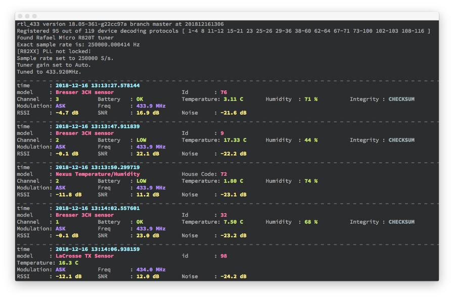
I. rtl_433
RTL_433 is an open-source software application used for receiving and decoding data from various wireless devices using RTL-SDR receivers including HackRF. It is primarily designed to work with inexpensive RTL2832-based DVB-T dongles that have been repurposed for general-purpose radio reception.
Here are some key points about RTL_433:
- RTL_433 is capable of decoding data from a wide range of wireless devices and protocols, including weather stations, temperature sensors, remote controls, doorbells, tire pressure monitoring systems, and more. It supports over a thousand different devices and protocols.
- RTL_433 works with RTL-SDR receivers, which are affordable USB dongles originally designed for digital television reception. These dongles can be modified to enable wideband radio reception, making them suitable for capturing signals from various wireless devices.
- RTL_433 can decode the data transmitted by wireless devices and provide information in a structured format. It can identify and interpret the sensor readings, device IDs, battery levels, and other relevant data contained within the received signals.
- The application provides multiple output options, such as displaying decoded data in the terminal/console, writing to log files, sending MQTT messages, and even publishing to an InfluxDB for integration with other applications or visualization tools.
- RTL_433 has an active community and is continuously being improved. The code is open-source, allowing users to contribute, add support for new devices or protocols, and customize the application according to their requirements.
- RTL_433 operates through a command-line interface, meaning it is primarily used via text commands in a terminal or console. This makes it suitable for integration with scripts, automation, and other applications.
RTL_433 is a powerful tool for capturing, decoding, and analyzing wireless data from a wide range of devices. It enables users to extract valuable information from signals transmitted by various wireless devices, providing opportunities for monitoring, automation, and data analysis.
3. Modulations
Imagine your smartphone with its diverse apps for gaming, music, and videos. Now, consider Software-Defined Radio (SDR) as an incredibly versatile radio equivalent that transforms its functions through software, akin to how your smartphone adapts with various apps.
Unlike traditional radios constrained by fixed hardware, SDR operates through software, either on a computer or specialized chip. This software guides the radio in switching frequencies and decoding received signals.
Visualize tuning in to your preferred radio station. While traditional radios have designated settings like AM or FM, SDR is like a virtual radio embedded in your device. Using software, you have the power to modify and tailor settings to receive any radio station, irrespective of being AM, FM, or digital.
Modulation in SDR is all about how the radio encodes and decodes information in the signals it receives. By changing the properties of these signals, like their amplitude (how strong they are), frequency (how fast they vibrate), or phase (where they start), it will help with representing the information to send. Modulation helps the SDR radio translate those signals into something understandable.
One popular modulation technique used in SDR is called “QAM” (Quadrature Amplitude Modulation). It’s like a way of packing more information into a signal by changing its amplitude and phase. Imagine you have a bucket of water, and you want to send a secret message to your friend using waves in the water. You have the ability to manipulate the size and shape of waves, and you can also initiate them from various points. Through this process, you can generate patterns that symbolize different letters or numbers. QAM applies a similar principle to radio waves, encoding information by altering the patterns of amplitude and phase changes.
In simpler terms, SDR modulation resembles an intelligent radio that utilizes software to tune into any radio station and decode the received signals into comprehensible information. It’s similar to having a radio that surpasses the capabilities of a standard one, as it can adjust and transform itself using software, much like a smartphone with its diverse range of applications.
Here are some of the most common ones:
- Amplitude Modulation (AM): This is a modulation technique where the strength or amplitude of a carrier signal is varied to transmit information. It is commonly used in broadcasting.
- Frequency Modulation (FM): In FM, the frequency of the carrier signal is changed based on the information being transmitted. It is known for its high-quality audio and is used in FM radio broadcasting.
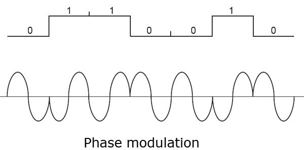
- Phase Modulation (PM): PM involves changing the phase of the carrier signal in response to the information being transmitted. It is used in various applications, including digital communication systems.
- Quadrature Amplitude Modulation (QAM): QAM is a type of modulation that combines both amplitude and phase modulation. It allows for the transmission of multiple bits of information simultaneously, making it efficient for high-speed data transmission, such as in Wi-Fi and cellular communication.
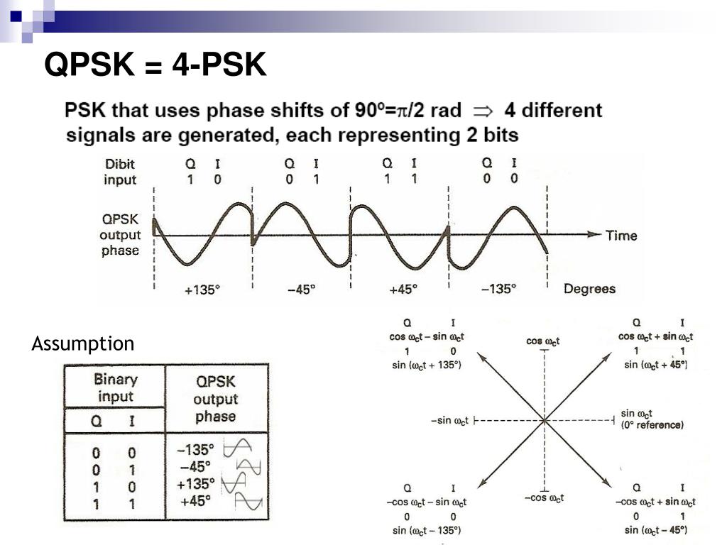
- Quadrature Phase Shift Keying (QPSK): QPSK is a digital modulation scheme where two bits of information are encoded in the phase of the carrier signal. It is widely used in satellite communication and digital broadcasting.
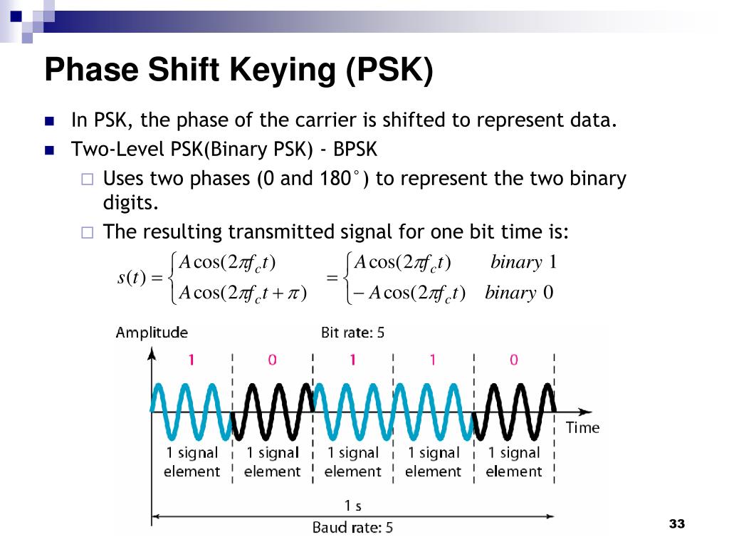
- Binary Phase Shift Keying (BPSK): BPSK is a type of modulation where the phase of the carrier signal is shifted to represent binary data. It is commonly used in wireless communication systems.
- Orthogonal Frequency Division Multiplexing (OFDM): OFDM is a multi-carrier modulation technique that divides the available frequency spectrum into multiple subcarriers. It is used in many modern communication systems, including Wi-Fi and 4G/5G cellular networks.
Let’s consider closely each on them.
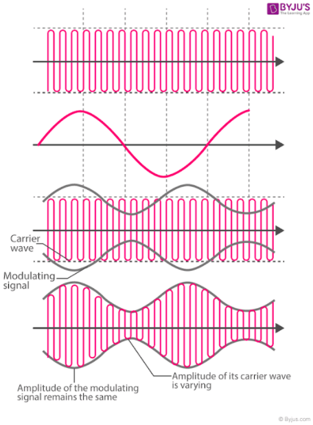
A. Amplitude Modulation
Amplitude Modulation (AM) is a method of encoding information onto a carrier signal by varying the strength or amplitude of the signal. It is commonly used in broadcasting, particularly in AM radio.
Imagine you have a carrier signal, which is like a steady “heartbeat” of a radio wave. It has a fixed frequency and carries no specific information on its own. The carrier signal is like a blank canvas waiting to be painted with the information you want to send.
To encode information using AM, you take the carrier signal and change its strength or amplitude according to the variations in the original signal you want to transmit. The original signal could be an audio sound, like a voice or music.
Here’s an analogy to help you understand it better: Imagine you have a light bulb that represents the carrier signal. It’s shining with a constant brightness. Now, imagine placing a piece of cardboard in front of the light bulb. By moving the cardboard closer or farther away, you can make the light appear brighter or dimmer.
In AM, the original signal (such as the audio) is used to control the cardboard, which represents the amplitude of the carrier signal. When the original signal is high or loud, it increases the amplitude of the carrier signal, making it brighter. When the original signal is low or soft, it decreases the amplitude, making it dimmer.
At the receiving end, another radio picks up the AM signal, and by detecting the variations in the carrier signal’s amplitude, it can recover the original signal. It’s like having someone on the other side who can watch the changes in the light bulb’s brightness and understand the hidden message.
AM allows us to transmit audio signals over long distances by piggybacking them onto carrier signals. This way, we can enjoy radio broadcasts, where voices, music, and other sounds are transmitted to our radios and played back for us to hear.
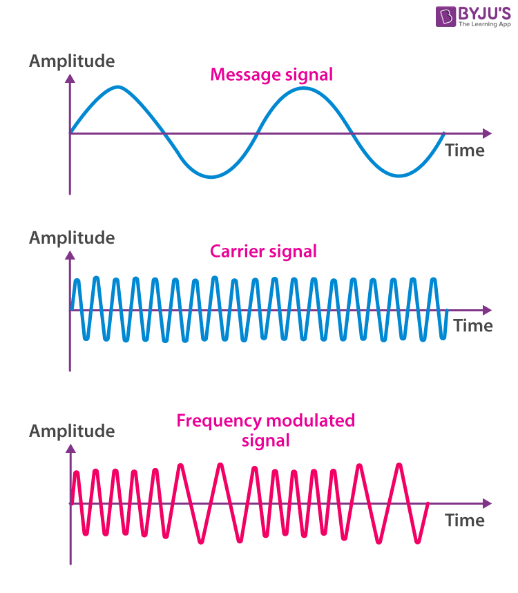
B. Frequency Modulation
Frequency Modulation (FM) is a method of encoding information onto a carrier signal by varying the frequency of the signal. FM is widely used in FM radio broadcasting and other communication systems.
Imagine you have a carrier signal, which is like a steady “heartbeat” of a radio wave with a fixed amplitude. In FM, instead of changing the amplitude like in AM, we modify the frequency of the carrier signal to represent the information we want to transmit.
Here’s an analogy to help you understand it better: Think of a playground swing. When you push the swing with a constant force, it swings back and forth at a regular speed. The speed of the swing is like the frequency of the carrier signal.
In FM, the original signal, such as an audio sound, controls how fast or slow the swing moves. When the original signal is high or loud, it increases the frequency of the carrier signal, causing the swing to swing faster. When the original signal is low or soft, it decreases the frequency, causing the swing to swing slower.
At the receiving end, another radio picks up the FM signal and detects the changes in the carrier signal’s frequency. By doing so, it can recover the original signal, such as the audio or music that was encoded onto the carrier signal.
FM is known for its high-quality audio transmission because it is less prone to noise and interference compared to AM. This is because the variations in the frequency of the carrier signal provide more robustness against disturbances in the transmission.
FM radio stations use this modulation technique to transmit music, voices, and other audio content. When you tune your FM radio to a specific station, you are selecting the carrier signal with a particular frequency that carries the desired information.
C. Phase Modulation
Phase Modulation (PM) is a method of encoding information onto a carrier signal by varying the phase of the signal. It is commonly used in digital communication systems and certain types of modulation, such as Quadrature Phase Shift Keying (QPSK) and Phase Shift Keying (PSK).
To understand phase modulation, let’s imagine a clock with a moving hand. The hand represents the carrier signal, and its position on the clock face represents the phase of the signal.
In PM, the original signal, such as an audio sound, controls the movement or rotation of the clock hand. When the original signal is high or loud, it rotates the clock hand faster, changing the phase more quickly. When the original signal is low or soft, it rotates the clock hand slower, resulting in a smaller change in phase.
At the receiving end, another device or radio detects the changes in the phase of the carrier signal. By measuring the difference in the phase from one moment to the next, it can recover the original signal.
Here’s an analogy to help you understand it better: Imagine you and a friend are sitting on a carousel. You both hold a flag, and as the carousel spins, you move your flag up and down. The position of your flag represents the phase of the carrier signal.
In PM, you and your friend can communicate by coordinating your flag movements. When you raise your flag high, it means one thing, and when you lower it, it means something else. By observing the changes in the relative positions of your flags, you can understand the message being conveyed.
Phase modulation is particularly useful in digital communication because it allows for efficient transmission of information. It can represent multiple bits of data simultaneously by dividing the phase into different states or symbols. This technique is used in various applications, including wireless communication, satellite communication, and digital broadcasting.
D. Quadrature Amplitude Modulation
Quadrature Amplitude Modulation (QAM) is a modulation technique that combines both amplitude modulation (AM) and phase modulation (PM) to encode information onto a carrier signal. It is widely used in digital communication systems, including Wi-Fi, cable TV, and cellular networks.
Imagine a graph with the horizontal axis representing the amplitude (strength) of the carrier signal and the vertical axis representing the phase (position) of the carrier signal. QAM uses this graph to encode multiple bits of digital information.
By varying both the amplitude and phase, QAM can create a constellation of points on the graph. Each point on the graph represents a specific combination of digital bits. The more points there are, the more information can be transmitted simultaneously.
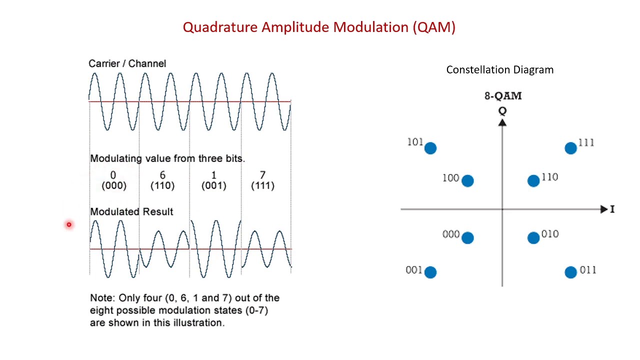
For example, a common form of QAM is 16-QAM, which uses 16 points on the graph. Each point represents a unique combination of four digital bits (2^4 = 16 possible combinations). Similarly, 64-QAM would use 64 points,
and so on.
At the receiving end, another device or radio detects the changes in both the amplitude and phase of the carrier signal and decodes the digital information based on the closest point on the graph.
QAM is used in various communication systems where high data rates are required. It allows for efficient transmission of large amounts of data over limited bandwidth, making it suitable for applications like high-speed internet access, digital TV, and mobile data communication.
E. Quadrature Phase Shift Keying
Quadrature Phase Shift Keying (QPSK) is a digital modulation scheme that is widely used in communication systems to transmit and receive digital data. It is a variant of Phase Shift Keying (PSK) modulation.
In QPSK, we take the concept of PSK and add another dimension to it. Instead of using just one carrier signal, QPSK uses two carrier signals, each shifted in phase by 90 degrees from one another. These two signals are often called the “in-phase” (I) and “quadrature” (Q) signals.
The QPSK modulation works as follows:
- Binary Data: The original digital data is grouped into pairs of bits. Each pair is represented by a symbol.
- Symbol Mapping: Each symbol is then mapped to one of the four possible phase shifts. These phase shifts are typically 0, 90, 180, and 270 degrees, corresponding to four points on a constellation diagram.
- Modulation: The in-phase (I) and quadrature (Q) carrier signals are each multiplied by the respective symbol to shift the phase of each carrier signal accordingly.
- Combination: The phase-shifted I and Q signals are then combined to create the QPSK signal.
At the receiving end, another device or radio receives the QPSK signal. It separates the combined signal back into the in-phase (I) and quadrature (Q) components. By comparing the phase of these components with the known constellation diagram, the original digital data can be decoded.
QPSK is efficient in terms of spectral efficiency because it transmits multiple bits per symbol. It is commonly used in applications such as satellite communication, wireless LANs (Wi-Fi), digital satellite TV, and cellular networks.
F. Binary Phase Shift Keying
Binary Phase Shift Keying (BPSK) is a digital modulation scheme that uses phase modulation to transmit binary (two-level) digital data over a carrier signal. It is a simple and commonly used modulation technique in digital communication systems.
In BPSK, the carrier signal is shifted between two possible phase states to represent the binary information. Typically, these phase states are 0 degrees and 180 degrees.
To understand BPSK, let’s consider a simple example:
- Binary Data: The original digital data consists of a sequence of binary bits, where each bit represents a 0 or a 1.
- Phase Mapping: Each bit is mapped to a specific phase shift of the carrier signal. For example, we can assign a phase shift of 0 degrees for a binary 0 and a phase shift of 180 degrees for a binary 1.
- Modulation: The carrier signal is then phase-shifted accordingly based on the binary data being transmitted. For each bit, the carrier signal is either left unchanged (0 degrees phase shift) or inverted (180 degrees phase shift).
- Transmission: The modulated signal, which alternates between two phase states, is transmitted over the communication channel.
At the receiving end, another device or radio detects the phase shifts in the received signal. By comparing the detected phase with the known phase shifts for binary 0 and 1, the original binary data can be recovered.
BPSK is often used in applications where simplicity and robustness are key factors. For example, it is commonly employed in satellite communication, digital data transmission over wired and wireless channels, and even in optical communication systems.
BPSK is relatively resilient to noise and interference, making it suitable for scenarios where signal quality might be compromised. However, it is less efficient in terms of bandwidth utilization compared to other modulation schemes that can transmit multiple bits per symbol, such as Quadrature Phase Shift Keying (QPSK).
G. Orthogonal Frequency Division Multiplexing
Orthogonal Frequency Division Multiplexing (OFDM) is a digital modulation and multiplexing technique used in communication systems to transmit multiple data streams simultaneously over a single communication channel. It divides the available frequency spectrum into multiple subcarriers that are orthogonal (independent) to each other.
To understand OFDM, let’s break down its key components and operation:
- Subcarrier Division: The available frequency spectrum is divided into a large number of narrow subcarriers. Each subcarrier occupies a specific frequency range within the overall spectrum.
- Orthogonality: The subcarriers are designed to be orthogonal to each other, meaning they don’t interfere with one another. This allows them to be closely spaced without causing interference or distortion.
- Data Encoding: Data to be transmitted is divided into parallel streams, each of which is assigned to a specific subcarrier. These streams can represent different users, data channels, or portions of the overall data transmission.
- Modulation: Each subcarrier is modulated independently using a modulation scheme like QAM or PSK. The modulation scheme determines how the data is encoded onto the subcarrier.
- Multiplexing: The modulated subcarriers are combined to create the composite OFDM signal. This composite signal contains all the individual subcarriers carrying different data streams.
- Transmission: The OFDM signal is transmitted over the communication channel, which could be wired or wireless.
At the receiving end, another device or radio receives the composite OFDM signal and performs the following steps:
- Demodulation: The composite signal is demodulated to extract the individual subcarriers.
- Channel Equalization: Each subcarrier is equalized to compensate for any distortions or interferences introduced by the communication channel.
- Decoding: Each subcarrier’s data is decoded, and the original data streams are reconstructed.
OFDM offers several advantages in communication systems:
- Efficient Spectrum Utilization: By dividing the available spectrum into numerous orthogonal subcarriers, OFDM maximizes the utilization of the frequency spectrum. This allows for high data rates and improved spectral efficiency.
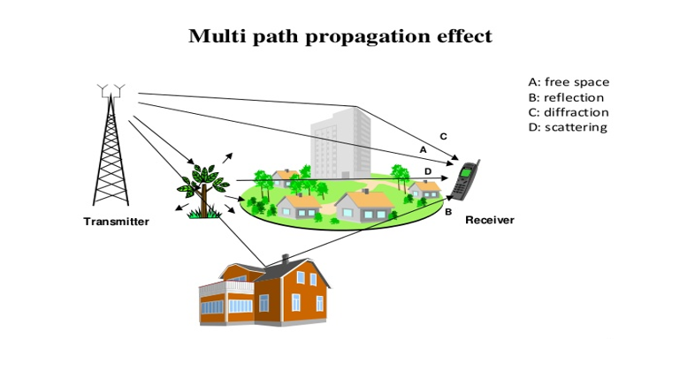
- Resistance to Multipath Fading: OFDM’s subcarriers are relatively narrow, making them less susceptible to the effects of multipath propagation. This improves the system’s resistance to fading caused by reflections and delays of the transmitted signal.
- Robustness to Interference: OFDM’s orthogonality between subcarriers provides inherent resilience to interference from adjacent channels or overlapping signals.
OFDM is widely used in various communication systems, including Wi-Fi (802.11a/g/n/ac/ax), 4G/5G cellular networks, digital television broadcasting (DVB-T/DVB-T2), and digital subscriber line (DSL) internet connections.
4. Radio waves
Before we move forward and dig into the real radio waves hacking, we have to discover one more crucial aspect – what is actually radio waves and how they work?
A. Radio waves explanation
Radio waves are a type of electromagnetic radiation with relatively long wavelengths and low frequencies. They are a form of energy that propagates through space in the form of oscillating electric and magnetic fields. Radio waves are commonly used for wireless communication, broadcasting, and various scientific and technological applications.
They are generated when charged particles, such as electrons, oscillate or accelerate in antennas and other devices. These oscillations create changing electric and magnetic fields that propagate through space.
Radio waves have several important characteristics that make them suitable for various applications:
- Long-range propagation: Radio waves can travel long distances, even over the curvature of the Earth. This property makes them ideal for long-distance communication and broadcasting.
- Penetration and diffraction: Radio waves can penetrate obstacles like walls and buildings, allowing them to be used for indoor communication. They also diffract around obstacles, which helps them reach receivers that are not in the line of sight.
- Wide range of frequencies: Radio waves span a broad spectrum of frequencies, ranging from a few kilohertz (kHz) to several gigahertz (GHz). This wide range enables different applications, such as AM/FM radio, television broadcasting, satellite communication, and wireless networks.
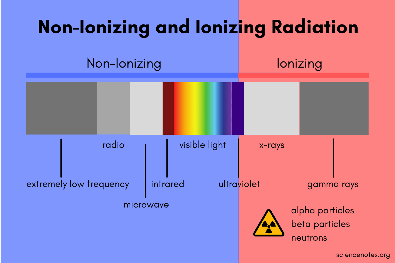
- Low energy and non-ionizing: Radio waves have relatively low energy compared to other forms of electromagnetic radiation, such as X-rays or gamma rays. They are considered non-ionizing, which means they do not have enough energy to remove electrons from atoms or molecules, making them generally safe for human exposure.
Let’s consider them one by one.
A.A. Long-range propagation
Long-range propagation refers to the ability of radio waves to travel over large distances, even beyond the line of sight between the transmitter and the receiver. This characteristic of radio waves allows for long-distance communication and broadcasting without the need for physical connections.
There are a few key factors that contribute to the long-range propagation of radio waves:
- Earth’s curvature: Radio waves can follow the curvature of the Earth, allowing them to propagate beyond the visual horizon. This is particularly important for applications like radio broadcasting, where signals need to reach listeners located far away from the transmitter.
- Ground wave propagation: At lower frequencies, typically below 2 MHz, radio waves can travel long distances by following the Earth’s surface. This mode of propagation is known as ground wave propagation. The radio waves interact with the Earth’s surface, causing them to bend and follow the curvature of the Earth. Ground wave propagation is often used in AM (Amplitude Modulation) radio broadcasting.
- Sky wave propagation: At frequencies above 2 MHz, radio waves can be reflected and refracted by the ionosphere—a region of the Earth’s upper atmosphere containing charged particles. This phenomenon, called sky wave propagation or ionospheric propagation, allows radio waves to be refracted back to the Earth’s surface, enabling long-distance communication. Sky wave propagation is utilized in shortwave broadcasting, amateur radio, and international long-distance communication.
- Tropospheric propagation: Within the lowest portion of the Earth’s atmosphere called the troposphere, radio waves can experience various propagation effects due to changes in temperature, humidity, and atmospheric conditions. These effects include tropospheric ducting, where the radio waves are trapped within a layer of the troposphere, enabling long-distance communication over bodies of water or across mountain ranges.
- Repeaters and relay stations: In cases where direct long-range propagation is not possible, intermediate relay stations or repeaters can be used to receive and retransmit the radio signals. These relay stations are strategically placed to extend the coverage range and ensure reliable long-range communication.
It’s important to note that the characteristics of long-range propagation can vary based on factors such as frequency, environmental conditions, atmospheric disturbances, and terrain. Different frequency bands exhibit different propagation properties, and the choice of frequency for a particular application depends on factors like desired range, available bandwidth, and environmental considerations.
A.B. Penetration and diffraction
Penetration and diffraction are two important characteristics of radio waves that contribute to their ability to propagate through obstacles and reach receivers even when there is no direct line of sight between the transmitter and the receiver.
Penetration: Radio waves have the ability to penetrate certain obstacles, such as walls, buildings, and foliage. The extent of penetration depends on the frequency of the radio waves and the nature of the obstacle. Lower frequency radio waves tend to have better penetration capabilities compared to higher frequency waves.
When radio waves encounter an obstacle, such as a wall, a portion of the wave’s energy can pass through the obstacle due to diffraction and the electromagnetic wave’s ability to couple with the conducting materials in the obstacle. The penetration ability of radio waves makes them suitable for indoor wireless communication, such as Wi-Fi networks, where signals can propagate through walls and other obstructions.
Diffraction: Diffraction is the bending and spreading of radio waves as they encounter an obstacle or pass through an opening that is comparable in size to their wavelength. When radio waves encounter an edge or an obstruction, such as a building or a mountain, they diffract around it, allowing the wave to reach areas that are beyond the direct line of sight.
Diffraction occurs because radio waves exhibit wave-like behavior, similar to other forms of waves. As the waves encounter an obstruction, they spread out, creating a pattern of secondary waves that propagate in different directions. This phenomenon allows radio waves to “bend” around corners and reach receivers that are not in the direct path of the transmitter.
The amount of diffraction depends on the wavelength of the radio waves and the size of the obstacle relative to the wavelength. Radio waves with longer wavelengths, such as those used in AM radio broadcasting, can diffract more readily around larger obstacles. In contrast, radio waves with shorter wavelengths, such as those used in Wi-Fi networks, experience more limited diffraction effects.
Diffraction is particularly important for radio waves in urban environments, where buildings and other structures can obstruct the direct line of sight between the transmitter and receiver. By utilizing the phenomenon of diffraction, radio signals can still reach receivers located behind buildings or around corners, enabling communication over a wider area.
Both penetration and diffraction play crucial roles in ensuring the reliability and coverage of radio communication systems. By allowing radio waves to propagate through obstacles and diffract around obstructions, they enable wireless communication in various scenarios and environments.
A.C. Wide range of frequencies
The wide range of frequencies refers to the broad spectrum of frequencies that radio waves can encompass. Radio waves span a wide range of frequencies, from the lower end of the electromagnetic spectrum to the higher end. This range allows for a diverse set of applications and technologies to operate within different frequency bands.
The frequency of a radio wave determines its characteristics, such as its wavelength, propagation characteristics, and the type of information it can carry. Here are some key frequency bands within the radio wave spectrum:
- Extremely Low Frequency (ELF) and Very Low Frequency (VLF): These frequency bands range from a few hertz to a few kilohertz. ELF and VLF waves are mainly used for communication with submarines, as they can penetrate seawater to reach submerged vessels.
- Low Frequency (LF) and Medium Frequency (MF): LF and MF bands span from kilohertz to a few megahertz. They are commonly used for AM radio broadcasting, navigation systems (such as the Non-Directional Beacon system), and maritime communication.
- High Frequency (HF): The HF band covers the range from a few megahertz to around 30 megahertz. HF waves can undergo sky wave propagation, where they are reflected and refracted by the ionosphere, enabling long-distance communication over continents or even across the globe. HF bands are utilized for shortwave broadcasting, amateur radio, aviation communication, and long-distance communication in remote areas.
- Very High Frequency (VHF) and Ultra High Frequency (UHF): VHF ranges from 30 megahertz to 300 megahertz, while UHF spans from 300 megahertz to 3 gigahertz. VHF and UHF bands are widely used for television broadcasting, FM radio, two-way radios, walkie-talkies, wireless microphone systems, and public safety communication.
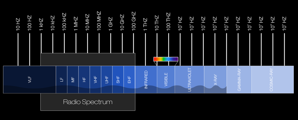
- Super High Frequency (SHF) and Extremely High Frequency (EHF): SHF ranges from 3 gigahertz to 30 gigahertz, and EHF spans from 30 gigahertz to 300 gigahertz. These high-frequency bands are utilized for various applications, including satellite communication, microwave links, radar systems, wireless local area networks (Wi-Fi), and 5G cellular networks.
The wide range of frequencies available for radio wave communication allows for different applications to operate in specific frequency bands that suit their requirements. Each frequency band has its own advantages and limitations in terms of propagation characteristics, signal penetration, bandwidth availability, and regulatory considerations. The allocation and usage of different frequency bands are typically regulated by government agencies to avoid interference and ensure efficient spectrum management.
A.D. Low energy and non-ionizing
Radio waves are characterized by their low energy compared to other forms of electromagnetic radiation, such as X-rays or gamma rays. This low energy level is an important characteristic of radio waves and contributes to their safety and non-ionizing nature.
Low energy: The energy of a radio wave is directly related to its frequency. Radio waves have relatively low frequencies compared to other types of electromagnetic radiation. The energy of a photon, which is a discrete packet of electromagnetic energy, is given by Planck’s equation: E = hf, where E represents energy, h is Planck’s constant, and f is the frequency of the wave. Since radio waves have low frequencies, the energy of their photons is correspondingly low.
Non-ionizing: The term “ionizing radiation” refers to forms of electromagnetic radiation that have enough energy to remove electrons from atoms or molecules, thereby ionizing them. Examples of ionizing radiation include X-rays, gamma rays, and some ultraviolet (UV) radiation. In contrast, radio waves do not possess enough energy to cause ionization. When radio waves interact with matter, they generally do not have the ability to break molecular bonds or produce ions.
The non-ionizing nature of radio waves is a significant factor in terms of their impact on biological tissues and their safety for human exposure. Unlike ionizing radiation, which can cause damage to cells and DNA, radio waves are considered to be biologically safe at typical exposure levels. This makes radio waves suitable for a wide range of applications, including wireless communication, broadcasting, and various technologies without posing significant health risks.
It’s important to note that while radio waves are non-ionizing and generally considered safe, very high power or prolonged exposure to radio waves can cause localized heating effects. This is the principle behind techniques like diathermy, which uses high-frequency radio waves for therapeutic heating in medicine. However, for typical everyday exposure levels to radio waves from common sources like Wi-Fi, mobile phones, and radio broadcasting, the energy is far below the threshold for causing significant heating or biological damage.
Regulatory bodies around the world, such as the Federal Communications Commission (FCC) in the United States, set guidelines and limits for exposure to radio waves to ensure public safety. These guidelines take into account the known biological effects and are designed to provide a margin of safety.
B. Radio waves length
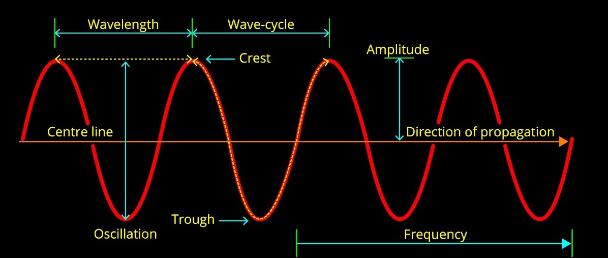
The length of radio waves is measured in meters (m) or multiples thereof, such as kilometers (km) or millimeters (mm), depending on their frequency. Since radio waves have a wide range of frequencies, their lengths can vary significantly.
Radio waves span a broad spectrum of frequencies, typically ranging from a few kilohertz (kHz) to several gigahertz (GHz). This frequency range corresponds to wavelengths ranging from hundreds of kilometers down to a few millimeters. The longer the wavelength, the lower the frequency and vice versa, according to the inverse relationship described by the equation:
c = λ * f
Where:
- c – represents the speed of light in a vacuum (approximately 3 x 10^8 meters per second)
- λ – represents the wavelength of the radio wave
- f – represents the frequency of the radio wave
For example, at a frequency of 1 megahertz (MHz), the wavelength is approximately 300 meters. At higher frequencies, such as 1 gigahertz (GHz), the wavelength becomes much shorter, around 30 centimeters.
Knowing the wavelength of radio waves is important for several reasons:
- Antenna design and performance: The design and performance of antennas depend on the wavelength of the radio waves they are intended to transmit or receive. Antennas are typically designed to be resonant at specific wavelengths to achieve efficient transmission or reception. By understanding the wavelength, engineers can design antennas that are properly matched to the desired frequency range, optimizing their performance and ensuring effective communication.
- Propagation characteristics: The wavelength of radio waves directly affects their propagation characteristics. Longer wavelengths tend to diffract more around obstacles, enabling them to propagate over longer distances and penetrate buildings more effectively. On the other hand, shorter wavelengths exhibit more directional propagation and are more susceptible to absorption and reflection by objects in their path. Understanding the wavelength helps in predicting how radio waves will behave in different environments, which is crucial for planning wireless communication systems and optimizing signal coverage.
- Frequency selection and interference avoidance: The wavelength is inversely proportional to the frequency of a radio wave. By knowing the wavelength, it becomes easier to determine the corresponding frequency or vice versa. This is important for frequency selection and coordination in various applications to avoid interference with other wireless systems operating in the same or nearby frequency bands.
- Regulatory compliance: Regulatory bodies, such as the FCC, allocate specific frequency bands for different applications and set limits on maximum allowed power levels. These regulations often refer to the wavelength or frequency range. Knowing the wavelength helps users and equipment manufacturers ensure compliance with regulatory requirements and adhere to the allocated frequency bands for specific applications.
- Compatibility and interoperability: Different wireless devices and systems operate within specific frequency ranges or wavelength bands. By understanding the wavelength, it becomes easier to assess the compatibility and interoperability of various devices and systems. For example, when integrating different wireless technologies or planning network deployments, knowledge of the wavelength helps ensure that the devices and systems operate within compatible frequency ranges to avoid interference and achieve seamless communication.
To better understand how it’s working, let’s calculate waves’ length for FM radio – 100 MHz, Smart Home – 433,92 MHz, Wi-Fi and GSM:
- Radio FM 100 MHz:
λ = (3 x 10^8 m/s) / (100 x 10^6 Hz)
λ = 300’000’000 / 100’000’000
λ = 3 meters
- Smart Home 92 MHz:
λ = (3 x 10^8 m/s) / (433.92 x 10^6 Hz)
λ = 300’000’000 / 433’920’000
λ ≈ 0.691 meters or 69.1 centimeters
- Wi-Fi: Wi-Fi operates in the 2.4 GHz and 5 GHz frequency bands. Let’s calculate the wavelengths for both:
For 2.4 GHz:
λ = 3 x 10^8 m/s / 2.4 x 10^9 Hz
λ = 300’000’000 / 2’400’000’000
λ ≈ 0.125 meters or 12.5 centimeters
For 5 GHz:
λ = 3 x 10^8 m/s / 5 x 10^9 Hz
λ = 300’000’000 / 5’000’000’000
λ ≈ 0.06 meters or 6 centimeters
- GSM: Global System for Mobile Communications operates in various frequency bands. Let’s calculate the wavelength for the most common GSM frequency band, which is 900 MHz:
λ = (3 x 10^8 m/s) / (900 x 10^6) Hz
λ = 300’000’000 / 900’000’000
λ ≈ 0.333 meters or 33.3 centimeters
C. Antennas’ types
We also calculate the length of radio waves to determine the appropriate antenna type and length. An antenna’s length is directly tied to the wavelength of the radio waves it’s intended to transmit or receive. Ensuring the antenna has the right length is crucial, as it guarantees optimal performance and efficiency in wireless communication.
The calculation of the correct antenna length depends on the type of antenna and the desired operating frequency. Different antennas have different formulas or guidelines for determining their optimal length. Here are a few examples of commonly used antenna types and their corresponding length calculations:
C.A. Dipole antenna (Half-Wave Dipole)
A dipole antenna, specifically a half-wave dipole antenna, is one of the most widely used and simplest antenna designs. It is a type of balanced antenna that consists of two conductive elements, each one-quarter of the wavelength in length, oriented in a straight line and separated by an insulator or a feed point.
- Structure: The half-wave dipole antenna consists of two conductive elements, typically made of metal, that are equal in length and symmetrically positioned. The length of each element is approximately one-quarter (1/4) of the wavelength of the desired operating frequency. The two elements are connected at their center by a feed point, where the antenna is connected to the transmission line or receiver.
- Resonance: The half-wave dipole antenna is designed to be resonant at its operating frequency. When the length of the dipole matches one-half of the wavelength, the antenna exhibits a resonant impedance, which allows for efficient energy transfer between the antenna and the transmission line or receiver.
- Radiation pattern: The radiation pattern of a half-wave dipole antenna is omnidirectional in the horizontal plane, meaning it radiates or receives signals equally in all directions around the antenna. The pattern is doughnut-shaped, with the maximum radiation occurring in the plane perpendicular to the antenna’s axis. In the vertical plane, the radiation pattern of a half-wave dipole antenna is more concentrated and varies depending on the height above the ground.
- Impedance: The characteristic impedance of a half-wave dipole antenna is typically around 73 ohms. This impedance can be matched to the impedance of the transmission line or receiver by using techniques like baluns or matching networks to minimize reflection and maximize power transfer.
- Applications: Half-wave dipole antennas find applications in various communication systems, including FM radio broadcasting, amateur radio, television reception, and wireless networks. They are also commonly used as reference antennas for testing and calibration purposes.
- Considerations: While the half-wave dipole antenna is relatively simple in design, it has a few important considerations. The physical length of the antenna must be accurately calculated or adjusted to match the desired operating frequency. The antenna should be mounted at an appropriate height above the ground, as the ground plane influences the antenna’s impedance and radiation pattern. Additionally, factors such as nearby objects, interference, and surroundings can affect the antenna’s performance, so careful placement and installation are important.
The half-wave dipole antenna offers a straightforward and efficient solution for various communication applications. Its simplicity, balanced structure, and omnidirectional radiation pattern make it a popular choice for many wireless systems.
The optimal length of a half-wave dipole antenna can be calculated using the formula:
Length (in meters) = (300 / Frequency in MHz) / 2
Basically, it’s the formula for calculation wavelength, divided by 2.
For example, if you want to design a half-wave dipole antenna for a frequency of 100 MHz, the calculation would be:
Length = (300 / 100) / 2 = 1.5 meters
It’s important to note that this and further calculations provide approximate lengths based on simple models and assumptions. In practice, other factors such as antenna structure, feeding methods, ground planes, and impedance matching techniques can influence the final antenna length. Additionally, real-world implementation may require adjustments or tuning to optimize the antenna’s performance.
C.B. Quarter-wave monopole antenna
A quarter-wave monopole antenna is a type of antenna that is widely used in various wireless communication applications. It is a variant of the dipole antenna and is often used when a ground plane is available.
The optimal length of a quarter-wave monopole antenna is calculated using the formula:
Length (in meters) = (300 / Frequency in MHz) / 4
For example, if you want to design a quarter-wave monopole antenna for a frequency of 433.92 MHz, the calculation would be:
Length = (300 / 433.92) / 4 = 0.173 meters or 17.3 centimeters
The quarter-wave monopole antenna offers a practical and efficient solution for a wide range of wireless communication applications. Its simplicity, compact size, and omnidirectional radiation pattern make it a popular choice in many wireless devices and systems.
C.C. Yagi-Uda antenna
The Yagi-Uda antenna, commonly referred to as a Yagi antenna, is a directional antenna widely used in applications that require high gain and focused signal radiation or reception in a specific direction. It was invented by Japanese engineers Hidetsugu Yagi and Shintaro Uda in the 1920s.
Here are some key features and characteristics of the Yagi-Uda antenna:
- Structure: The Yagi-Uda antenna consists of several elements arranged in a specific pattern. The main elements include a driven element, a reflector, and one or more directors. The driven element is the active component that is directly connected to the transmission line, while the reflector and directors act as passive elements that enhance the antenna’s performance.
- Directionality: The Yagi-Uda antenna is highly directional, meaning it focuses its radiation or reception in a specific direction. The reflector element is positioned behind the driven element, while the directors are placed in front of the driven element. This configuration causes the antenna to emit or receive signals with maximum gain in the forward direction and reduced gain in other directions.
- Gain: The Yagi-Uda antenna is known for its high gain, which is achieved by the combination of the driven element, reflector, and directors. The reflector element enhances the antenna’s directivity by reflecting the signals toward the driven element, while the directors help to further concentrate the energy in the desired direction. The gain of the Yagi-Uda antenna depends on factors such as the number of directors, spacing between elements, and their lengths.
- Radiation pattern: The Yagi-Uda antenna exhibits a highly focused radiation pattern with a narrow beam width in the forward direction. The beam width determines the angular coverage over which the antenna radiates or receives signals effectively. The radiation pattern of the Yagi-Uda antenna is asymmetric, with the maximum radiation occurring in the direction of the directors and reduced radiation in other directions.
- Limitations: While the Yagi-Uda antenna offers high gain and directivity, it is primarily designed for a specific frequency or narrow frequency band. Changing the operating frequency significantly can affect the antenna’s performance. Additionally, the antenna’s performance is affected by factors such as nearby objects, ground plane, and surrounding environment, so careful installation and positioning are important.
Designing a Yagi-Uda antenna involves considering various parameters such as element lengths, spacing, and element diameter. Optimization is crucial to achieve the desired gain, directivity, and radiation pattern. Simulation software and design tools are commonly used to model and analyze the antenna’s performance to achieve optimal results.
The Yagi-Uda antenna is widely used in various applications, including television reception, point-to-point communication links, amateur radio, Wi-Fi networks, and direction finding systems. Its directional properties and high gain make it suitable for scenarios where long-range communication, signal concentration, or interference rejection is desired.
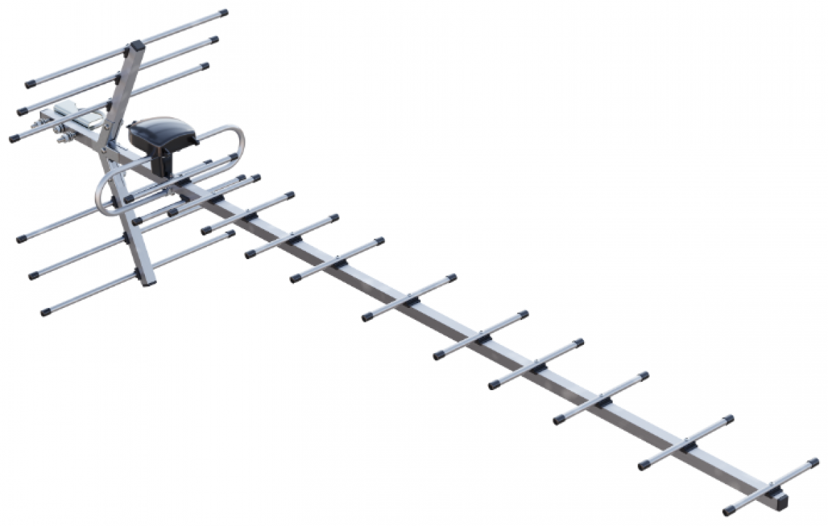
C.D. Patch antenna
A patch antenna is a flat antenna commonly used in applications like Wi-Fi or GPS. The optimal length of a patch antenna depends on its design, substrate properties, and desired frequency. Designing a patch antenna often requires simulations and specialized software tools to achieve the desired performance.
Here are some key points about patch antennas:
- Structure: A patch antenna consists of a radiating patch element printed on a dielectric substrate and a ground plane on the opposite side of the substrate. The patch is usually a conductive metal trace, such as copper, etched on a substrate material like FR4. The shape of the patch can vary, with rectangular and circular patches being the most common.
- Planar design: Patch antennas are planar antennas, which means they are relatively flat and thin. This planar design allows for easy integration into devices, printed circuit boards (PCBs), or other planar surfaces, making them suitable for compact and low-profile applications.
- Resonance: The patch antenna operates at its resonant frequency, which is determined by the dimensions of the patch element and the dielectric substrate. The resonant frequency is typically in the microwave or higher frequency ranges. By adjusting the dimensions of the patch and the substrate, the resonant frequency can be tuned to match the desired operating frequency.
- Radiation pattern: The radiation pattern of a patch antenna can vary depending on the specific design and shape of the patch element. In general, patch antennas exhibit a relatively wide radiation pattern in the plane of the patch (broadside) and a narrow radiation pattern in the direction perpendicular to the patch (end-fire). However, the radiation pattern can be modified through various techniques, such as adding additional elements or using specialized feed structures.
- Gain and efficiency: Patch antennas can achieve moderate to high gain depending on their design and size. The gain is influenced by factors such as the size of the patch, the substrate thickness, and the dielectric constant of the substrate material. Efficiencies of patch antennas can also be quite high when designed and implemented properly.
- Feeding techniques: Patch antennas can be fed using different techniques, including microstrip feed, coaxial feed, aperture-coupled feed, or proximity-coupled feed. The choice of feeding technique depends on the desired impedance matching, ease of fabrication, and performance requirements.
- Applications: Patch antennas find applications in various wireless systems, including wireless communication, navigation systems, satellite communication, radio frequency identification (RFID), and IoT devices. They are commonly used in devices like smartphones, tablets, laptops, wireless routers, and RFID readers, where compact size and good performance are important.
- Design and optimization: Designing a patch antenna involves considering various parameters, such as the patch size, substrate material, substrate thickness, feed location, and impedance matching techniques. Simulation software and design tools are commonly used to model and analyze the antenna’s performance and optimize its characteristics.
Patch antennas offer several advantages, including their compact size, ease of integration, planar structure, and moderate to high gain. Their versatility and performance make them a popular choice in many wireless communication applications, where space constraints and performance requirements are critical factors.
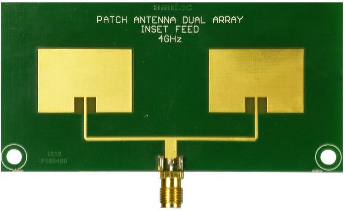
D. Placing the antenna
When it comes to placing an antenna, there are several key rules to consider optimizing its performance and ensure effective communication.
For antennas that rely on direct line-of-sight (LOS) communication, such as point-to-point microwave links or satellite dishes, it is essential to have a clear and unobstructed path between the transmitting and receiving antennas. Obstructions like buildings, trees, or other structures can attenuate or block the signal, leading to reduced performance or complete signal loss.
Placing the antenna at an appropriate height is crucial for maximizing its range and coverage. Higher placement generally provides a better line of sight, reduces interference from ground-level objects, and minimizes signal blockage. The height will depend on the specific application and the surrounding environment.
Ensure the antenna is securely mounted and stable to prevent movement or misalignment due to wind, vibrations, or other external factors. Proper mounting ensures that the antenna maintains its optimal orientation and alignment for effective communication.
Avoid placing the antenna in close proximity to objects that can interfere with its signal, such as large metallic structures, power lines, or other antennas. These objects can introduce interference or cause signal reflections that affect the antenna’s performance.
Proper grounding of the antenna is important for safety reasons and to protect against electrical surges or lightning strikes. Follow the manufacturer’s guidelines and local regulations for proper grounding techniques.
Consider the polarization of the antenna and ensure it aligns with the polarization of the desired signal source or target antenna. Proper alignment helps maximize signal reception or transmission.
If possible, place the antenna away from sources of electromagnetic interference (EMI) to minimize signal degradation. EMI sources include power lines, motors, high-voltage equipment, or other devices that emit electromagnetic noise.
Pay attention to the routing and length of the coaxial cable connecting the antenna to the receiver or transmitter. Use appropriate cable lengths and quality to minimize signal loss and maintain the antenna’s performance.
Take into account the environmental conditions that may affect the antenna’s performance. Factors such as wind, temperature variations, precipitation, and exposure to sunlight can impact the antenna’s durability and signal quality. Choose antennas designed to withstand the specific environmental conditions of the installation site.
Saying that, placing the antenna outside a building or car is important. First of all, it’s avoiding signal blockage. Buildings and vehicles can act as significant obstacles that block or attenuate radio waves. Radio waves have difficulty penetrating through the walls, roof, and windows of buildings, as well as the metal body of a vehicle. By placing the antenna outside, you can avoid or minimize the blockage caused by these obstacles, allowing for better signal reception or transmission.
Following that, placing the antenna outside provides a clearer line of sight to the signal source or target. As mentioned earlier, line of sight is essential for optimal wireless communication. By positioning the antenna outside, you can reduce the number of obstructions between the antenna and the desired signal, improving the strength and quality of the received or transmitted signal.
Next, inside buildings or vehicles, there may be various sources of electromagnetic interference, such as electronic equipment, power lines, or other wireless devices. These sources can introduce noise and distort the signal, affecting the overall signal quality. By moving the antenna outside, you can reduce the proximity to potential sources of EMI and minimize their impact on the signal.
Also, radio waves propagate differently indoors compared to outdoor environments. Indoor environments are characterized by more signal absorption, reflections, and signal degradation due to the presence of walls, furniture, and other objects. By placing the antenna outside, you can take advantage of the more favorable propagation characteristics of open spaces, where signals can propagate over longer distances and with reduced interference.

5. Analyze the spectrum
Let’s start our practical part and the only right point to begin with is to scan our neighborhood.
To do that we will use the hackrf_spectrum_analyzer application discovered previously. To install that just download the latest release from the official GitHub – https://github.com/pavsa/hackrf-spectrum-analyzer/releases, unpack and then just launch the bash script.
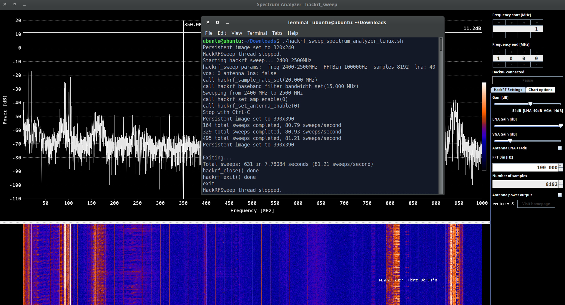
We limited our radio waves range scan from 1 MHz to 1 GHz but it was more than enough for our research purposes. Before we take a closer look at our graphs let’s make some settings adjustments. First of all, we would suggest to scroll up the waterfall graph so we can see the spectrum’s history (it’s more important rather than a current rapidly changing graph).
Next, switch on the “Show peaks” item (under “Chart Options” folder) so we can determine our neighborhood radio spectrum.
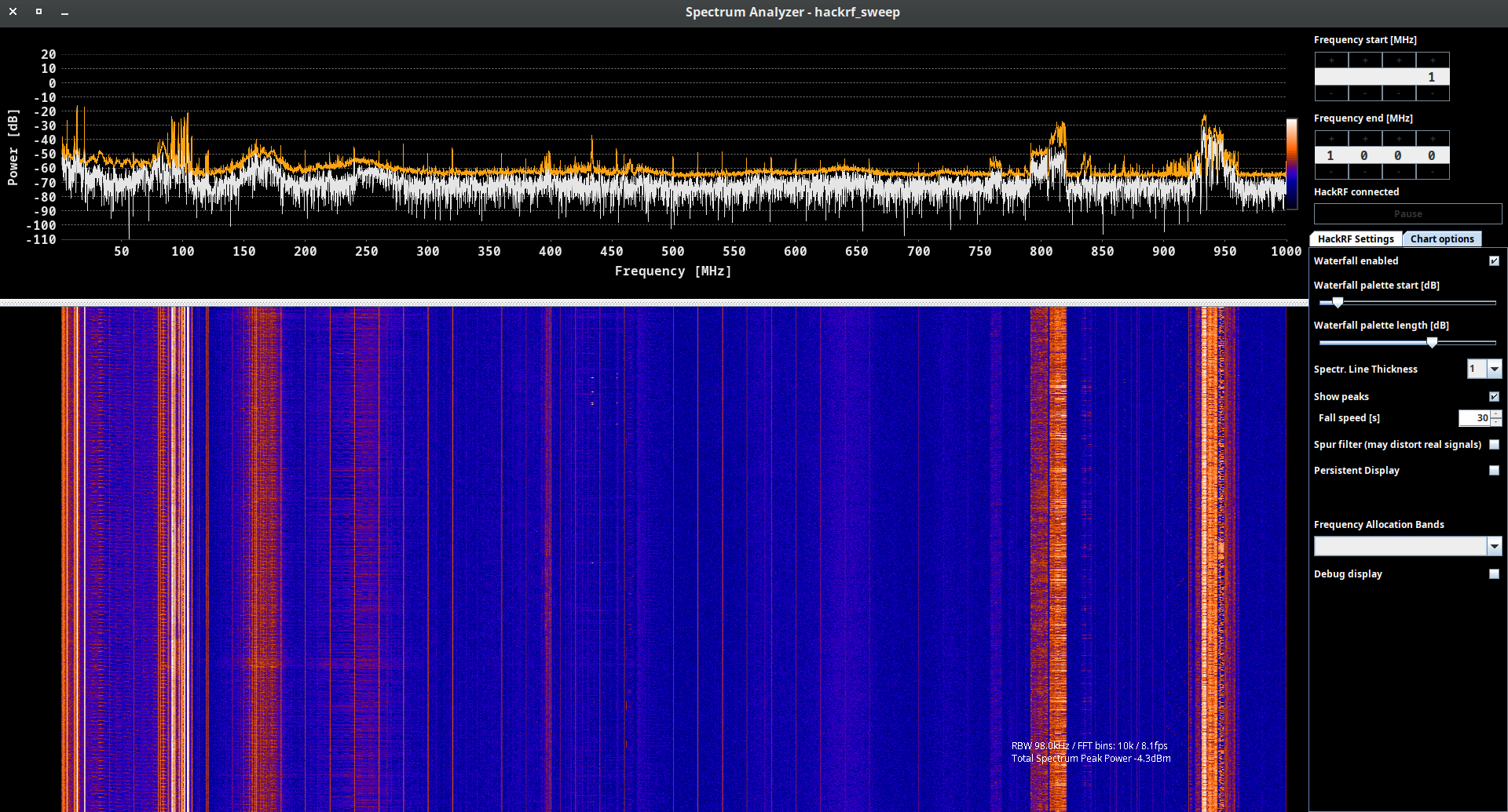
By the way, it’s quite useful feature in case you are in charge of against or looking for eavesdrop equipment. Imagine, you are monitoring your company’s area and suddenly find out there is some powerful 108 MHz transmitting going from CFO’s office which started right after the business partner arrived.
It’s not rare that business reconnaissance is masquerading under a valid stuff and radio waves are not an excluding. And if we are talking about 108 MHz FM transmitter, there is no need for a special receiver – just a simple radio: in car or Android phone, portable radio, etc.
The last item is adjusting some filters regarding Gain and WaterFall pallets so you can clearly see the payload signal and sort it out from the noise.
A. 1-50 MHz
Now let’s consider our neighbor’s spectrum from left to right. As you can see there are some strong signals from 1 till roughly 50 MHz so we have to look closer to it.
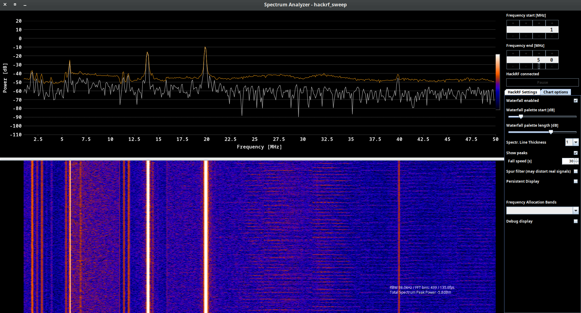
We can find out there are some super powerful peaks like 5.5, 13.5 and 20 MHz as well as 2, 3 and 40. But do you know what is working on those frequencies? This frequency range is often referred to as the “medium frequency” and “high-frequency” bands. Different applications and services utilize different parts of this spectrum. Here are some of the main uses:
- The AM radio broadcast band falls within the MF range, typically between 540 kHz and 1600 kHz (1.6 MHz). This is where you find traditional AM radio stations.
- Shortwave broadcasting occurs in the HF range, typically between 2 MHz and 30 MHz. These frequencies can travel long distances via ionospheric propagation and are used for international broadcasting and reaching remote areas.
- The amateur radio service operates in various bands throughout the 1 MHz to 50 MHz range. Different portions of the spectrum are allocated for different types of communication (e.g., voice, data, Morse code) and for different classes of amateur radio operators.
- CB radio operates in the HF band between 26.965 MHz and 27.405 MHz. It is commonly used for short-range, personal communication, often in vehicles or for hobbyist purposes.
- Some specific frequencies within this range are used for marine and aviation communication, particularly for long-range communication over water and remote areas.
- Certain frequencies within this range are allocated for radio control of model aircraft, boats, cars, and other remote-controlled devices.
- Some navigation systems, such as LORAN-C (Long Range Navigation System), once used frequencies within this spectrum, though many of these systems have been phased out in favor of GPS.
- Some portions of the spectrum are reserved for emergency communications, public safety organizations, and disaster relief operations.
- Telemetry systems, which transmit data wirelessly, can also operate in various parts of this frequency range.
B. 80-130 MHz
Next range is somewhere between 80 and 130 MHz, but as you may guess mostly it’s simple Radio FM stations. The FM radio broadcast band falls within the VHF range, typically between 88 and 108 MHz. Regardless what city or country you are right now, that range is locked/registered for civil radio stations.
For instance, here you can find almost all FM Radio stations the US – https://radio-locator.com/.
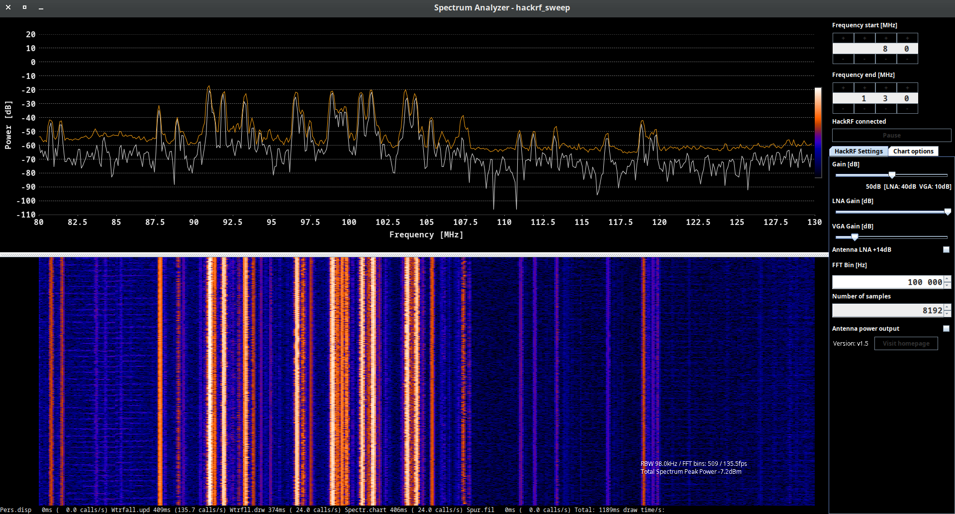
C. 150-180 MHz
Another valuable range is between 150 and 180 MHz. Plenty of services are working on these frequencies, including amateur radio, VHF FM radio broadcast auxiliary services, land mobile communication, radio astronomy and telemetry, satellite and aircraft communications. But for our region the marine communication is the main one. We will discover that further in the current book.
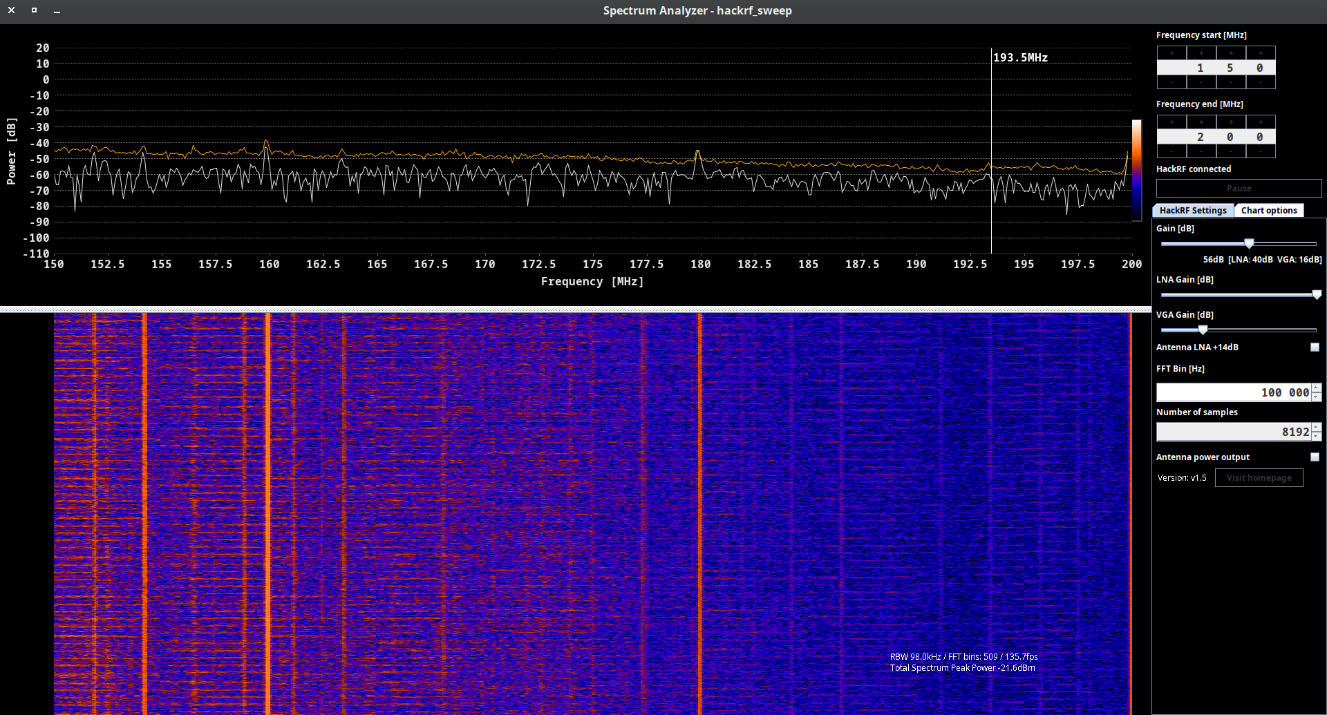
D. 430-480 MHz
Now, we would suggest to skip a big bunch of range and look closer to the most interesting items from 430 to 480 MHz.
First of all, we need to know what is 433.92 MHz range. That radio spectrum is commonly used for various wireless communication and remote control applications, especially in the field of short-range devices:
- Remote Keyless Entry (RKE): Many modern vehicles use the 433.92 MHz frequency for keyless entry systems. When you press a button on your car key fob to lock or unlock your vehicle, it typically uses this frequency to communicate with the car’s receiver.
- Wireless Doorbells: Some wireless doorbell systems operate at 433.92 MHz. When the doorbell button is pressed, it sends a signal to the doorbell chime, producing the ringing sound (we will talk about wireless doorbell hacking further).
- Wireless Alarms and Security Systems: Some alarm and security systems utilize the 433.92 MHz frequency for wireless communication between sensors and the central control unit.
- Remote Controls for Electronics: Some consumer electronics, such as garage door openers, remote-controlled toys, and home automation devices, use this frequency for wireless remote control.
- Wireless Weather Stations: Some wireless weather monitoring stations and sensors operate at 433.92 MHz to transmit weather data to a central receiver or display unit (we will talk about Wireless Weather Stations hacking further).
- Wireless Sensor Networks: In some cases, wireless sensor networks use the 433.92 MHz spectrum for transmitting data from various sensors, such as temperature sensors, humidity sensors, and motion detectors.
- Radio-Controlled Clocks: Some radio-controlled clocks and watches use the 433.92 MHz frequency to synchronize the time with a centralized time signal.
- Home Automation: Some home automation systems use the 433.92 MHz spectrum for controlling lights, switches, and other smart home devices.
But why that frequency is so popular and widely used? The use of the 433.92 MHz frequency has several advantages for certain wireless communication and remote control applications. Here are some of the key advantages:
- License-Free Spectrum: In many parts of the world, the 433.92 MHz frequency band is designated as a license-free Industrial, Scientific, and Medical (ISM) band. This means that devices operating within this frequency range do not require individual licenses for use, making it easier and more cost-effective for manufacturers to implement wireless communication solutions.
- Good Range: The 433.92 MHz frequency has relatively good propagation characteristics. It can penetrate walls and obstacles better than higher-frequency bands, allowing signals to travel over a reasonable range in indoor and outdoor environments.
- Low Power Consumption: Devices operating at 433.92 MHz can be designed to consume relatively low power, which is especially beneficial for battery-operated devices like remote controls, key fobs, and sensors. Lower power consumption leads to longer battery life and reduced maintenance.
- Simple Antennas: Antennas operating at lower frequencies are generally more manageable in size and design. This simplicity can help reduce the size and cost of devices, making them more compact and attractive to consumers.
- Wide Availability of Components: The 433.92 MHz frequency is widely used in various consumer and industrial applications, leading to a broad range of available components and off-the-shelf solutions. This availability simplifies the design and manufacturing process for devices operating at this frequency.
- Reduced Interference: Compared to higher-frequency bands, the 433.92 MHz spectrum is less crowded, leading to reduced chances of interference from other devices operating in the vicinity. This can improve the reliability and performance of wireless communication systems.
- Compatibility with Legacy Devices: Many existing remote control and wireless devices operate at 433.92 MHz. As a result, new devices designed for this frequency can be backward compatible with older devices, ensuring seamless integration and easy replacement.
- Cost-Effectiveness: Due to the license-free nature of the 433.92 MHz band and the wide availability of components, devices operating at this frequency are often more cost-effective to manufacture, making them attractive for mass-market consumer products.
Despite these advantages, it’s important to note that the 433.92 MHz frequency also has limitations. Its lower data transmission rates compared to higher-frequency bands can restrict its use in applications that require high data throughput. Additionally, as an unlicensed band, there can be a risk of potential interference from other devices operating in the same frequency range.
Now let’s come back to our graph. As you can see there is some transmitting at 433.92 MHz range which means we have some “Smart Home” device next to us. What is that – doorbell, weather station, car key, etc. – we don’t know yet, but we will definitely reveal.
The great stuff if it’s weather station hence we can “steal” the payload and get our own weather station for free.
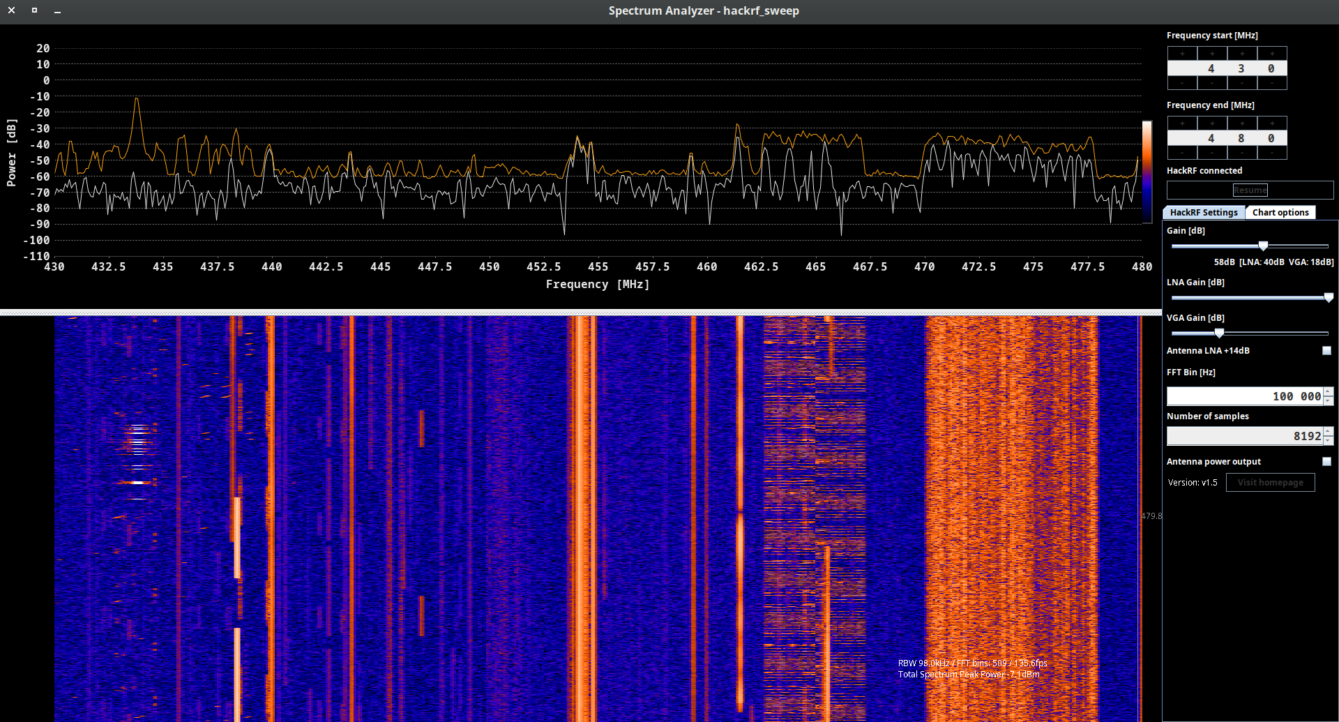
Except Smart Home devices we have some occasional transmitting between considering range. Most probably there are walkie-talkies, wireless microphones, radio control and hobbyist devices. There are vast variety of possibilities and each particular case has to be investigated what we will do in the next chapter.
E. 790-960 MHz
The radio spectrum from 790 MHz to 960 MHz covers a range of frequencies that is commonly used for various communication and broadcasting applications, especially in the context of mobile communication and wireless networks. This frequency range is often referred to as the “800 MHz band” and the “900 MHz band.” Here are some of the main uses of the 790 MHz to 960 MHz radio spectrum:
- Cellular Mobile Communication: The 800 MHz and 900 MHz bands are historically significant for the development of cellular mobile communication systems. They have been used for various generations of mobile networks, including 2G (GSM), 3G (UMTS/WCDMA), and early 4G (LTE) networks.
- Public Safety Communication: In some countries, portions of the 800 MHz band have been allocated for public safety communication systems, such as police, fire, and emergency services.
- Private Mobile Radio (PMR): Certain segments of the 800 MHz and 900 MHz bands are allocated for private mobile radio systems, which are used by businesses, industries, and other organizations for internal communication.
- Wireless Data Communication: The 900 MHz band, in particular, has been utilized for wireless data communication and internet services, especially in areas where wired broadband infrastructure is limited.
- Wireless Local Area Networks (WLAN): Some countries have allocated specific frequency bands within this range for WLAN use, including Wi-Fi networks operating in the 900 MHz ISM band.
- RFID (Radio Frequency Identification): Certain RFID systems operate in the 900 MHz band, particularly in the range of 902 MHz to 928 MHz, which is allocated as an ISM band in some regions.
- Broadcasting: Some countries have allocated certain frequencies within the 790 MHz to 862 MHz range for terrestrial digital television broadcasting.
It’s important to note that the specific frequency allocations within the 790 MHz to 960 MHz spectrum can vary by country and region. The usage of this spectrum is heavily regulated by national regulatory authorities to avoid interference and ensure efficient use of the limited frequency resources.
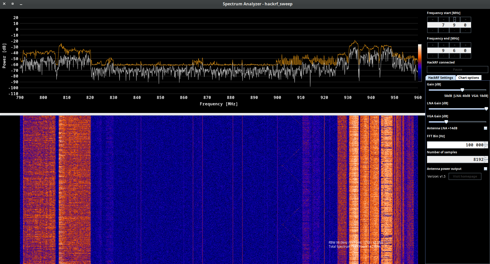
F. Alternatives
As an hackrf_spectrum_analyzer alternative you can use any of SDR applications, for instance CubicSDR which we will widely use further. You can not only watch the range and analyze it, but also listen the channel if it’s transmitting the sound.
But there is a significant drawback of all of that kind of apps. If you wanna use it as a spectrum analyzer – the sample rate is limited up to 20 million samples per second.
It means you can see and work only with 20 MHz range, e.g. from 88 till 108 MHz, from 430 till 450 MHz or, what is more crucial, only from 2400 till 2420 MHz.
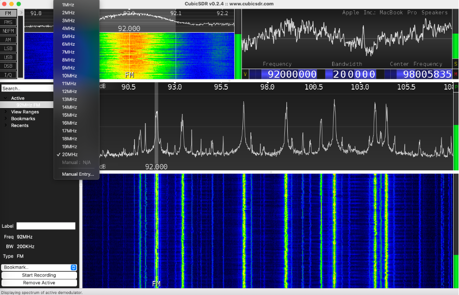
So, the point is to choose the proper application wisely, based on your real needs.
6. Playing with signals
Having analyzed the spectrum, we are ready to go into analyzing signals. We will try to listen the payload (if possible), get ships and boat GPS coordinates, receive the temperature and many other things. Let’s not waste any time and dig into.
A. Listen to the radio
We’ll begin with the most straightforward exercise, attempting to tune in to the radio, often referred to as the “Hello World” in the SDR community. To get started, connect your HackRF to your PC and open your preferred SDR application. We will explore various programs, and we’ll begin with CubicSDR.
A.A. CubicSDR
After launching the CubicSDR, we have to choose the SDR device and in our case it’s HackRF One #0.
As we discussed previously, Radio FM bands are between 88 and 108 MHz band hence let’s set it up by choosing the frequency somewhere between that range, e.g. 92 MHz (space key). Don’t forget to adjust the sample rate and set it up to 10 MHz.
So, take the FM modulation, hover your mouse over the peak and click. If you did everything correct you have to listen the radio.
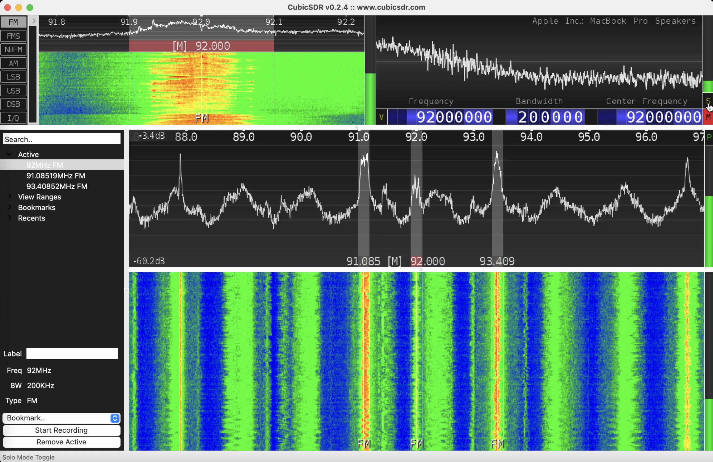
One of the features of CubicSDR is you can listen several frequencies at the same time. Just keep the Shift key pressed down and chose the peak. In our example we listened ~91.1 MHz, 92 MHz and ~93.4 MHz together.
Indeed, and we agree with you, for Radio it’s not so convenient to listen several bands due to its mess and not understandable, but in a moment we will proof you it’s the important stuff.
A.B. SDRangel
Next, let’s do the same exercise using SDRangel app. That won’t be as easy as we’ve done with CubicSDR, but manageable. We hope you have already plugged in your HackRF so let’s just launch it.
Once it’s opened, we have to choose “Add RX device” from the top menu. Unfortunately, it does not have any shortcuts or downlist in main menu hence you have to memorize icons’ images and their order.
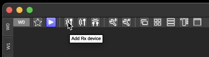
Having clicked the button, the app would ask you to select sampling device; in our case it’s HackRF[0]. 2 additional windows have to appear on your workspace.
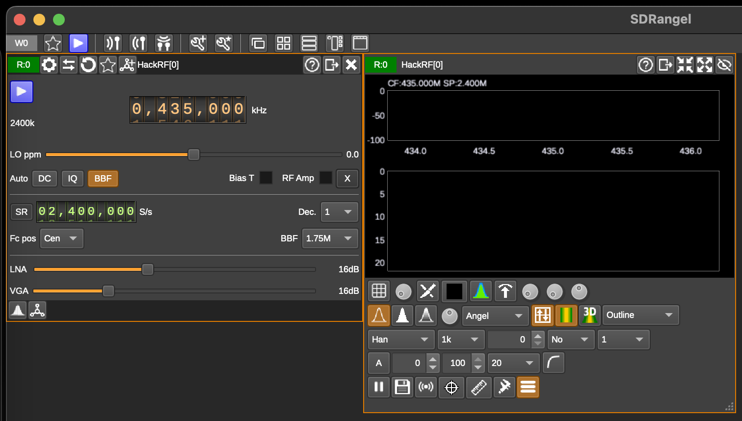
So, the left window is in charge of adjusting settings like frequency, decimation factor, RF bandpass filter, auto correction and other. The right one is just a spectrum visualization.
Next, we need to set up a modulation onto wide FM. To do that click “Add channels” icon…
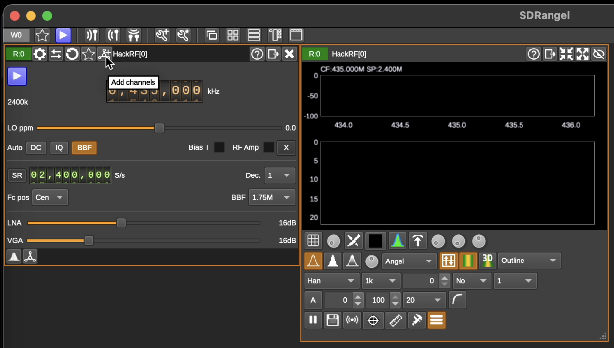
and choose “WFM Demodulation”.

The new window “WFM Demodulation” has to appear.
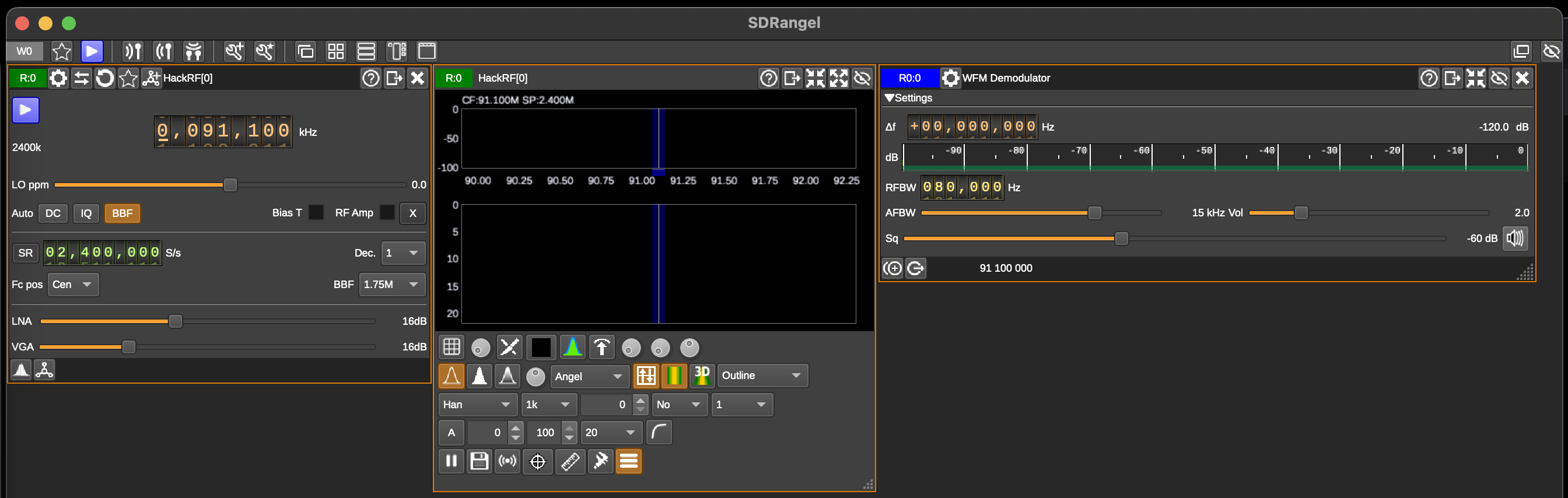
In the following image, you’ll discover the ideal settings to listen to the radio.
However, you might be somewhat taken aback because nothing seems to be occurring. It’s perfectly normal to be surprised by this lack of activity. To make it function properly, we need to raise both the LNA and VGA levels and adjust the RFBW to 200,000 Hz. Only after making these adjustments you will be able to hear clear and loud sound. In the following image, you’ll discover the ideal settings to listen to the radio.
In the following image, you’ll discover the ideal settings to listen to the radio.
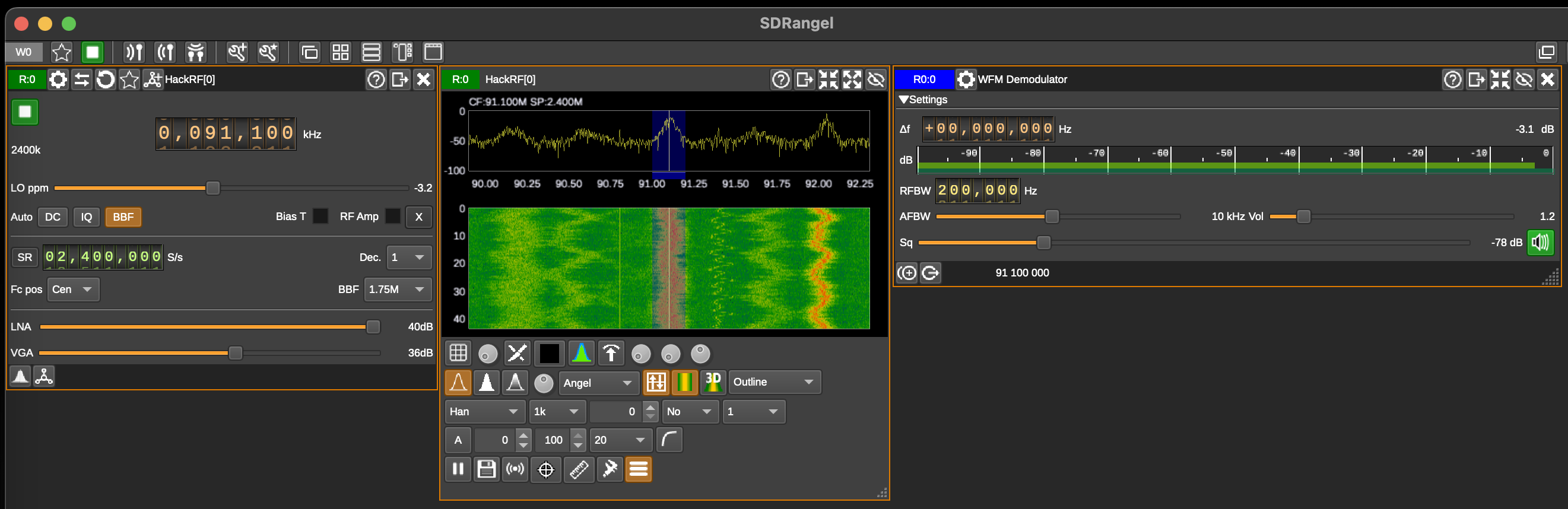
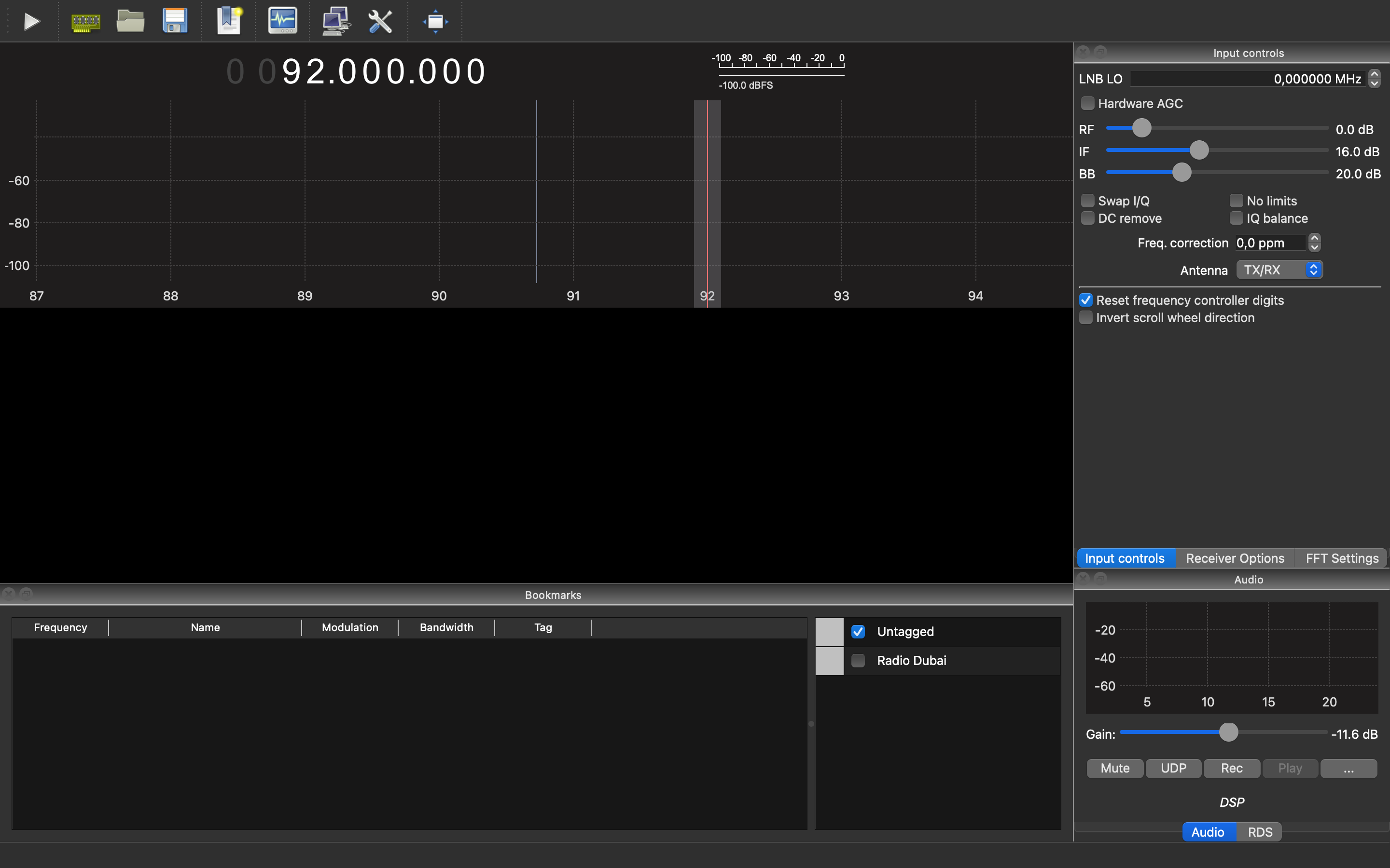
One outstanding feature of this program is that GQRX automatically detects connected devices like HackRF, RTL-SDR, and others. Therefore, if you launch GQRX after connecting your HackRF, there’s no need to manually select the correct device—it’s already configured by the application.
Let’s delve into how it operates. When you open it, you should see a window similar to the one in the previous picture: with graph and waterfall sections, a bookmarks window on the left, and various settings on the right.
The numbers, as seen in CubicSDR and SDRangel, are expressed in GHz, MHz, KHz, and Hz, respectively. You can adjust these values using your mouse or by directly entering the numbers from your keyboard.

To listen the radio, except the frequency, we have to implement several settings like “Filter width” – Wide, and “Mode” – “WFM (mono)”.
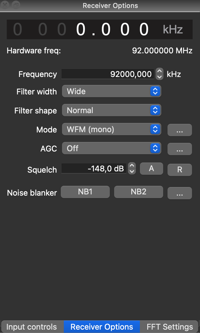
So, if you did everything correctly, having pressed the “Start DSP” button you have to listen the signal.
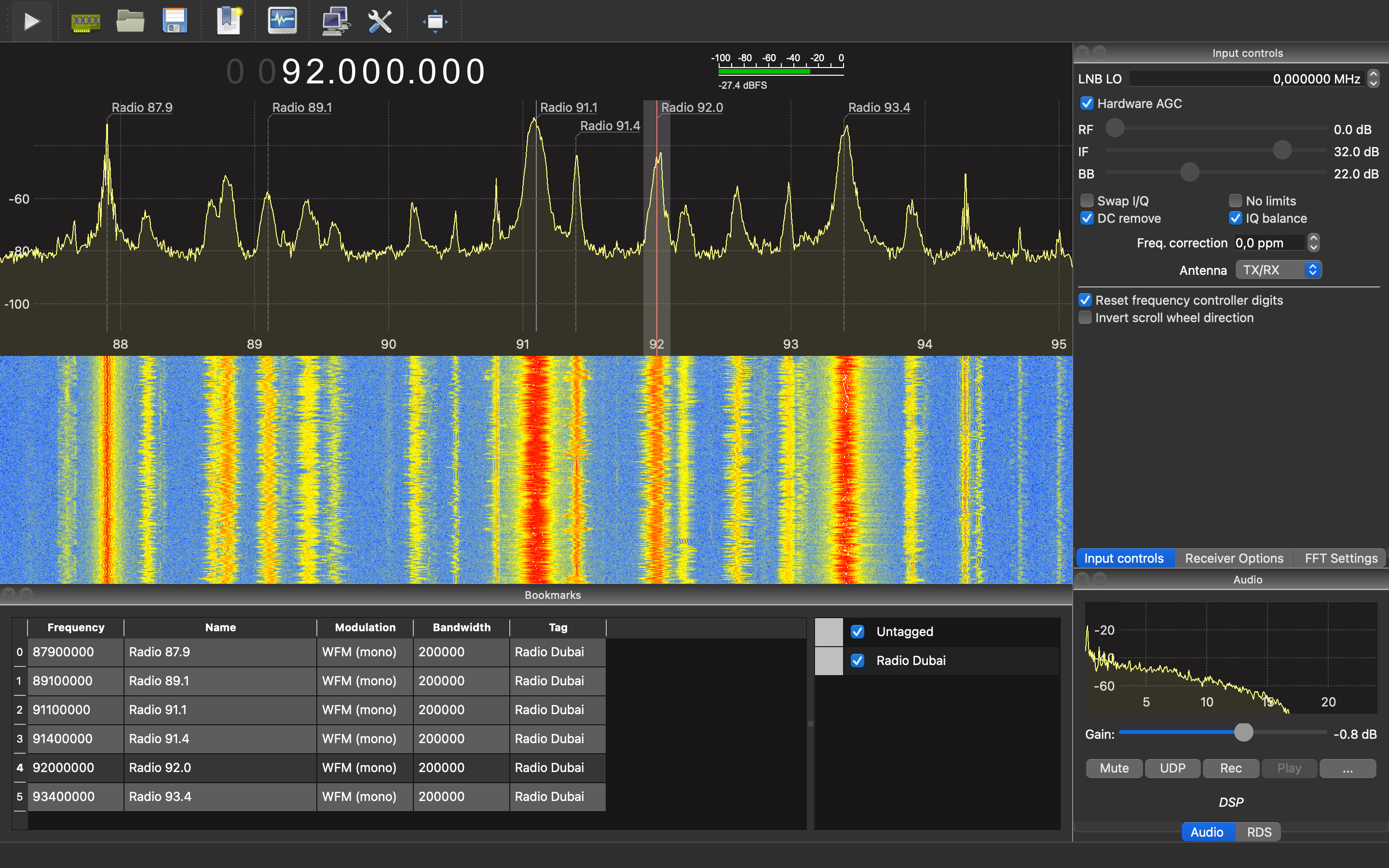
One additional feature which you can see on the screen as well as in the video – bookmarks. Indeed, CubicSDR has the same functional, but… GQRX is allowing you to label each frequency and put it on the graph for your convenient jumps between stations.
A.D. GNU Radio Companion
If we can consider SDR apps as program languages, in that case CubicSDR and GQRX will be like Scratch, SDRanges – Python, but GNU Radio – C/C++.
Which means you have to have deep knowledges of SDR, radio waves and physics overall.
In essence, it functions like a constructor, yet the sequence in which you arrange the blocks is of utmost importance. Initially, it might seem overly intricate and perhaps unnecessary, especially when we have other user-friendly high-level applications available. However, once you become proficient with it, you’ll realize that CubicSDR and similar tools only tap into about 10% of what GNU Radio is capable of.
Is it truly necessary? Well, that depends on your specific requirements, but we strongly recommend gaining at least a basic understanding of it.
For the best GNU Radio learning resources, you can check out the tutorials provided by Michael Ossmann, the founder of HackRF, on his YouTube channel – https://www.youtube.com/@GreatScottGadgets. You will learn not only about GNU Radio, but digital signal processing, decibels, complex numbers, HackRF one by itself and many more other related and needed things.
Because the charter is about listen to the radio, let’s create a GNU Radio graph to catch some music. How to do that, Michael is describing at his first video – https://www.youtube.com/watch?v=BeeSN14JUYU.
You can download the final GNU Radio graph from his web-site https://greatscottgadgets.com/sdr/1/ – lesson1.grc (For GNU Radio v3.9 onwards) and launch that.
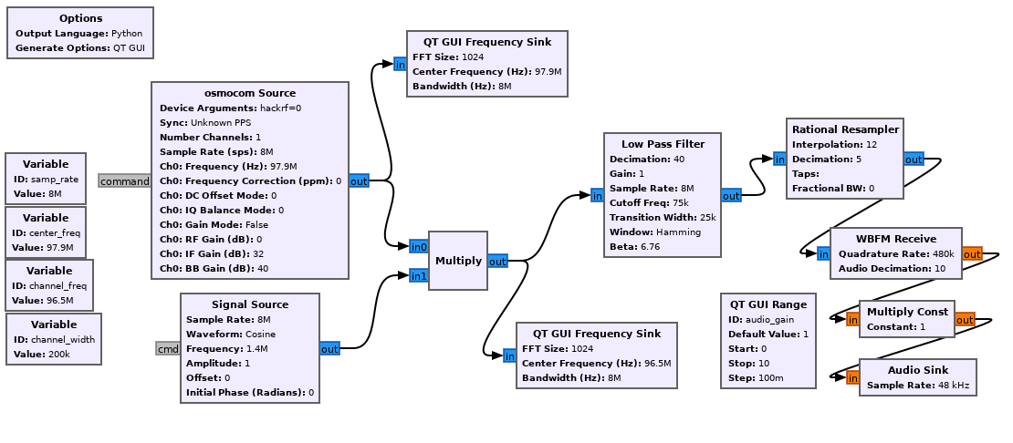
That will work perfectly. However, there is room for enhancements to make it more user-friendly. Additionally, we don’t want to merely mimic Michael’s work like script kiddies. Let’s enhance the graphical representation.
To begin, the most straightforward change is to remove the initial “QT GUI Frequency Sink.” Initially, it was included to verify the correct functioning of everything. However, now that the graph is properly configured, having an extra frequency sink graph appears unnecessary.
Another drawback is that we can change the frequency only when the app is stopped. Let’s fix that so we can adjust the frequency any time during its running. To aim that we need to add another one “QT GUI Range”. Set the ID as “channel_freq”, label as “Frequency”, Default_value as 91.1e6 (which basically means 91.1 multiply by 1’000’000 or 91.1 MHz), Start and Stop as 88e6 and 108e6 respectively, and the Step as 1e5 (0.1 MHz).
In that case we no need anymore the static “channel_freq” variable hence it can be deleted.
As the final step we need to beatify the Volume range label. Open the “audio_gain” QT GUI Range and set the Label as “Volume”.
If you did everything correct, you have to get the next graph:
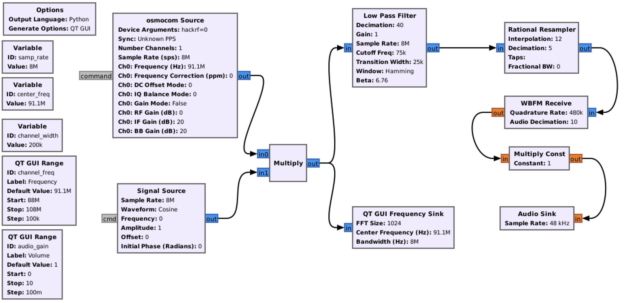
After executing the flow graph we have to hear the radio sound. Let’s check.
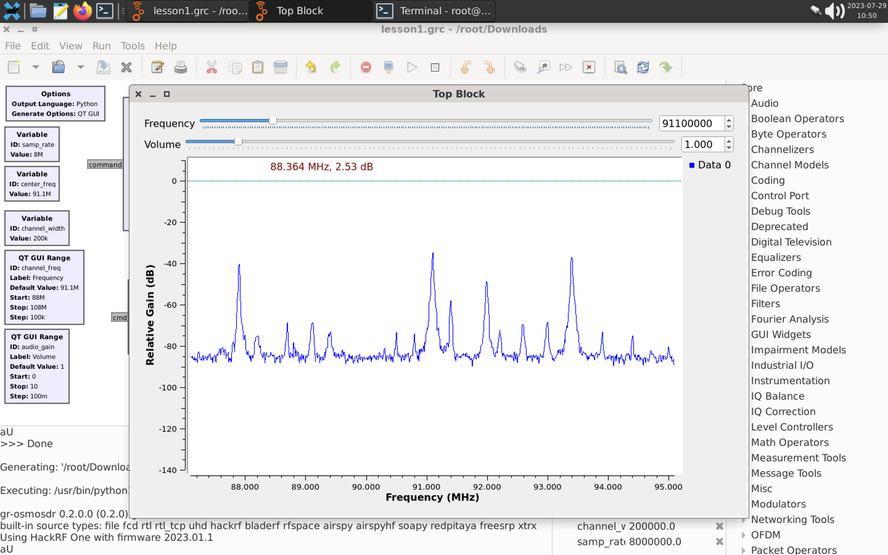
After executing the flow graph we have to hear the radio sound. Let’s check.
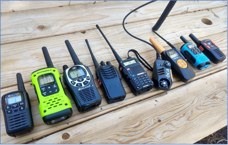
Walkie-talkies are used in a variety of settings, such as outdoor activities (they are popular among hikers, campers, and adventurers who need reliable communication in areas without cell phone coverage), construction and industrial sites (workers at construction sites, factories, and large industrial complexes use walkie-talkies to coordinate tasks and ensure safety), events and festivals (organizers of events and festivals use walkie-talkies to coordinate logistics and ensure smooth operations) and, the most important, security and emergency services (law enforcement, security personnel, and emergency responders use walkie-talkies for quick and efficient communication during operations).
Walkie-talkies usually work on 2 set of frequencies:
- VHF walkie-talkies operate within the frequency range of approximately 136 to 174 MHz
- UHF walkie-talkies operate within the frequency range of approximately 400 to 470 MHz
The common modulation is Narrow FM, but sometimes we can meet AM.
Having known that, let’s try to intercept some signals.
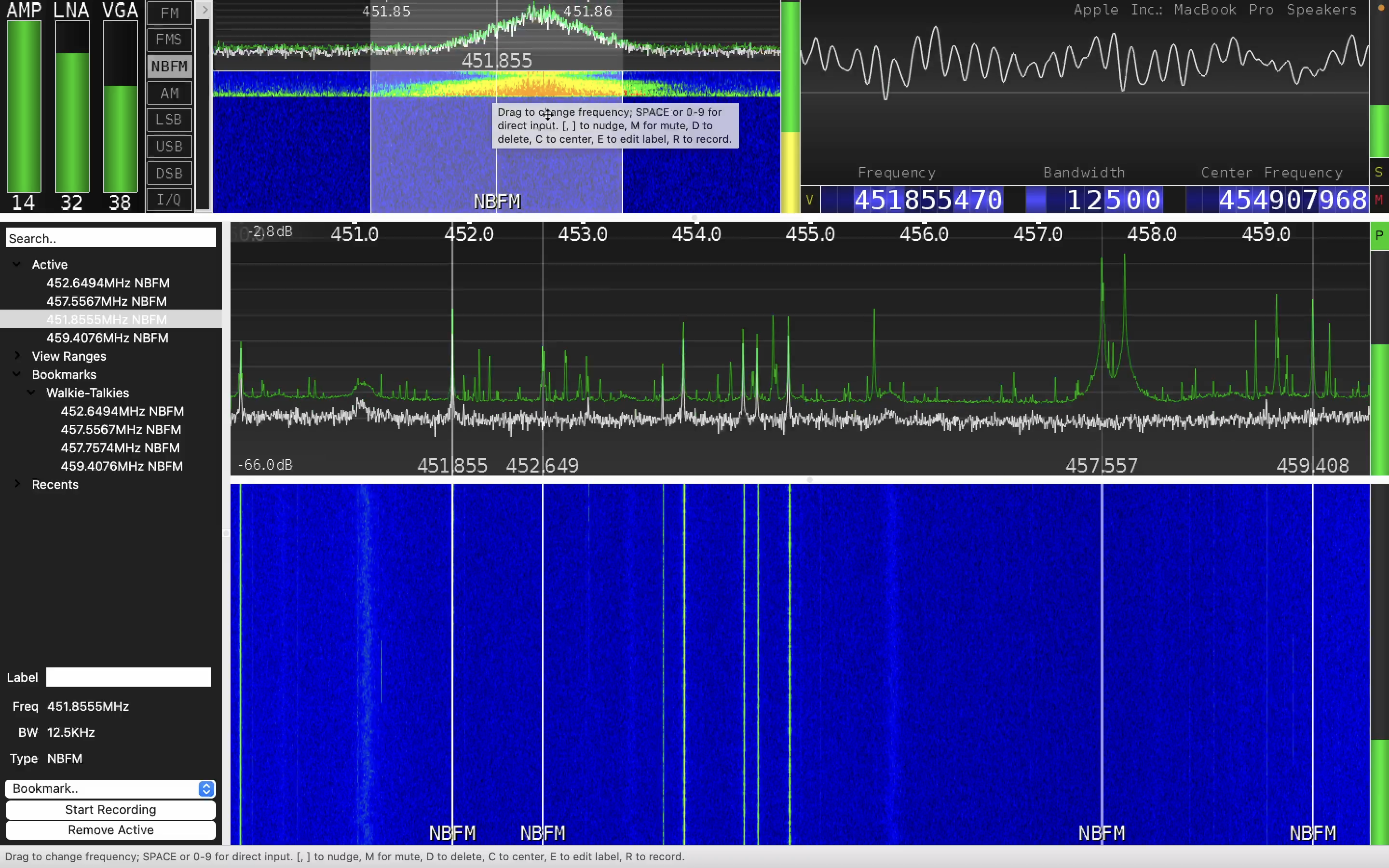
Basically, as you can see, the approach is 100% the same as listening the Radio hence just set up the proper frequency and the modulation.
But let’s consider that deeply – from the security perspective. Due to the fact that mostly all of walkie-talkie’s communications are not encrypted at all, it’s a significant security flaw. Moreover, if you purchase the same radio station as your “victim”, you can easily listen to him/her and even trick by transmitting the fake data.
So, if we are talking about hiking with friends and using a clear text communication – it’s an acceptable risk. Moreover, in case of emergency you can share the SOS signal and get help.
But now transfer that flaw into law enforcement and security guards staff? Each your correspondence with departments or between officers is “open to the world”. Back to our home countrythe majority of law enforcement agencies were utilizing APCO P25 modulation. This meant that if you had the appropriate software demodulator, you could listen in on police communications regarding various incidents such as car accidents and domestic violence. Remember those scenes in movies where reporters sit in their cars, listening to police radios to arrive at a crime scene and write their articles? Well, for us, that wasn’t a movie plot; it was our reality.
As Red Teamers, our primary focus is on security personnel. Understanding that businesses often view their security departments as cost centers and prioritize price in procurement decisions, the equipment used is often inexpensive and lacks adequate protection. During Red Team activities, it becomes crucial to ascertain if you’ve been detected and gather other vital information. Furthermore, by employing HackRF as a transmitter (as discussed later in our book), you can pose questions, deceive security personnel with false information (“Team, we have a security breach at gate 2. Immediate backup required.”), or disrupt their communications by generating white noise on their channel.
C. Marine tracks
Each ship and even boat across the globe must have a radio station with some kind of GPS tracking. It is mandatory by regulators and forced by security reasons. Communication, emergency and distress calls, weather information, navigation aids, maritime safety information, communicating with onshore facilities, crew welfare – it’s far away not the full list of reasons why the radio station is implemented in every marine stuff.
Following those items, marine transactions, including GPS coordinates, are not closed or private. In the maritime industry, vessel positions and certain transactional information are often publicly available and shared through various means.
While certain sensitive information related to the ship’s crew, cargo details, or commercial contracts may not be publicly disclosed, vessel positions and basic transactional data are generally accessible to various stakeholders involved in the maritime industry.
It’s worth noting that data privacy and security are essential considerations in the modern maritime world. Vessel tracking data is often collected by Automatic Identification System (AIS) and transmitted over public channels. However, there are efforts to ensure that this data is not misused and that sensitive information is appropriately protected. Additionally, technology advancements and regulatory changes might have occurred after issuing that article, so it’s always good to verify the current practices and regulations in the maritime industry.
Marine radio communications operate on specific frequency bands that are reserved for maritime use. The primary frequency bands used for marine communication are within the VHF (156.000 to 162.025 MHz) and HF (1.605 to 27.500 MHz) ranges. These frequencies allow for reliable short to medium-range communication over water.
There is a website called VesselFinder (https://www.vesselfinder.com/) where you can find any global ship’s photos, position, track, tonnage and other relative data.
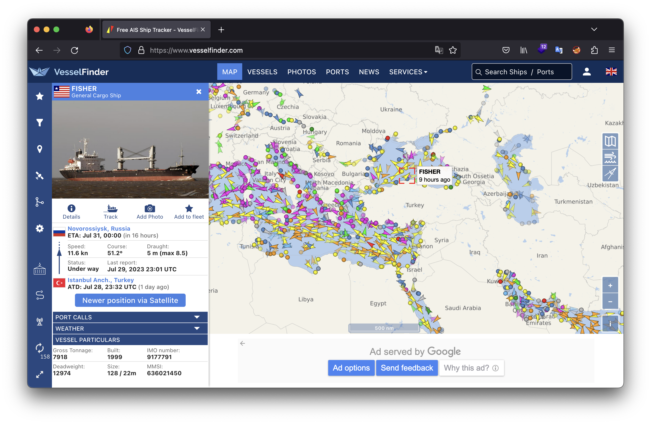
We believe that we’ve covered sufficient theory, and now it’s time to engage in some hands-on research. Fortunately, we have a nearby seaport, allowing us to admire some “such a pretty boat… ship” as Captain Jack Sparrow would say.
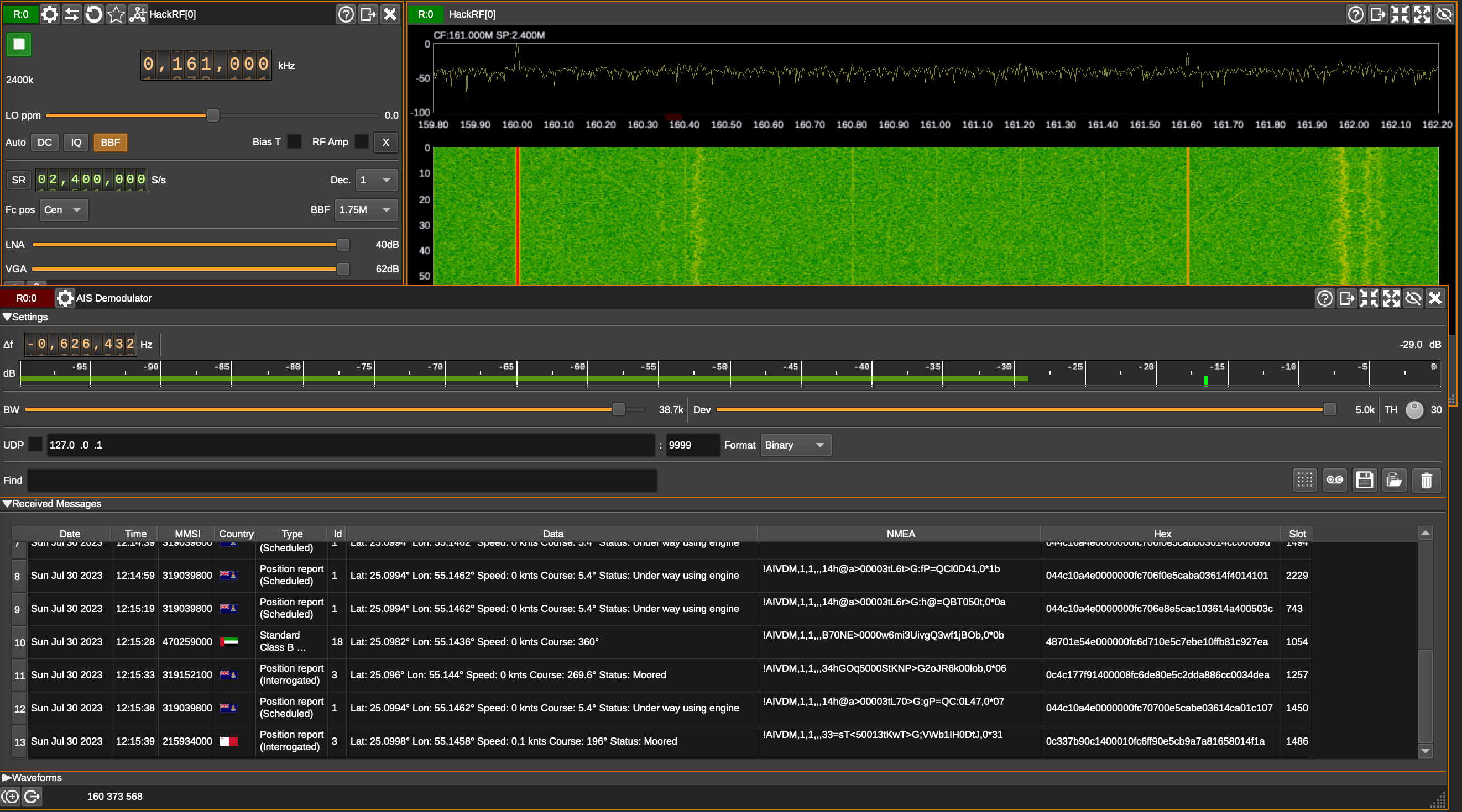
Launch your SDRangel, set up the frequency as 160.373.600 Hz (our case) and add new channel as “AIS Demodulator”. In a moment your AIS Demodulator window will be started fulfilling by ships’ data.
The great feature of that app is that if you double click to MMSI, the new browser window will be opened with the respected data about the Yacht.
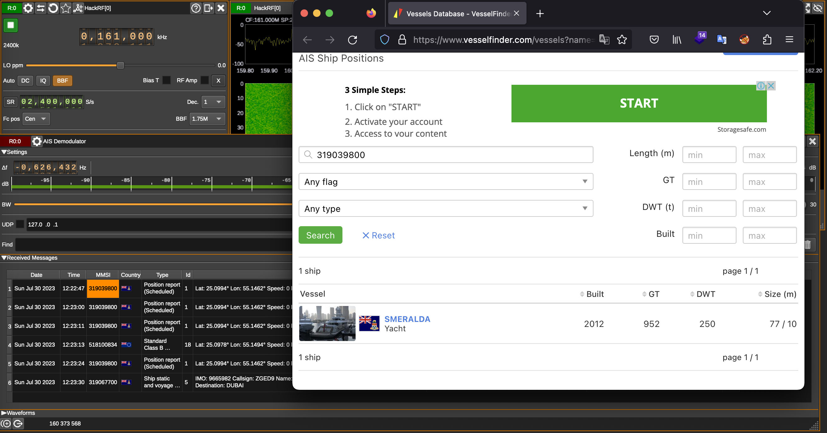
D. White noise (Wi-Fi Jammer)
White noise is a type of noise signal that contains all frequencies in equal proportions, making it sound like a constant and uniform hissing or static sound. It is called “white” noise because it is analogous to white light, which contains all colors in the visible spectrum in equal amounts.
In technical terms, white noise is a random signal with a flat power spectral density. This means that it has an equal amount of energy at all frequencies within a specified range. As a result, it has a constant power across the entire frequency spectrum.
White noise is often used in various applications, including audio engineering, acoustics, signal processing, and scientific research. Some common uses of white noise include:
- Sound Masking: White noise is used to mask or cover up background sounds, creating a more peaceful or private environment. For example, white noise machines are often used in offices or bedrooms to drown out distractions or aid in sleeping.
- Testing and Calibration: In scientific experiments and measurements, white noise can be used to test and calibrate various equipment and systems.
- Signal Processing: White noise is used as a reference signal in certain signal processing applications, such as testing audio equipment or analyzing the frequency response of a system.
- Random Number Generation: White noise is employed in some algorithms to generate random numbers for simulations and other computational purposes.
From the security perspective and, what is more important, Red Team point of view, what noise can perform positive services as well as breaching your perimeter.
If we are talking about legal use of white noise, it’s often related to such kind of closed rooms for negotiations; dealing with state’s secret documents; prisons; to land the drone, etc. If you need to be sure, that your conversation is private and kept in secret, you can install a respected equipment to jam radio channels as well as turn down Dictaphone’s microphone.
From the Red Teamer’s perspective, we can use it to block closing gates, steel the flying drone or jam Wi-Fi signal. Making a long story short, let’s create a white noise to cover our personal Wi-Fi signal and make a Wi-Fi Jammer.
First, let’s remember what frequencies Wi-Fi is working on and how it’s divided. Wi-Fi is working on 2.4 GHz frequency and consists of 14 channels of 22 MHz each.
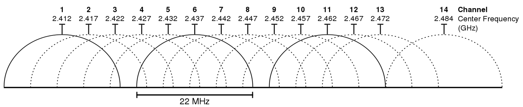
Channel Identifier | Center Frequency (MHz) | Range (MHz) |
1 | 2412 | 2401–2423 |
2 | 2417 | 2406–2428 |
3 | 2422 | 2411–2433 |
4 | 2427 | 2416–2438 |
5 | 2432 | 2421–2443 |
6 | 2437 | 2426–2448 |
7 | 2442 | 2431–2453 |
8 | 2447 | 2436–2458 |
9 | 2452 | 2441–2463 |
10 | 2457 | 2446–2468 |
11 | 2462 | 2451–2473 |
12 | 2467 | 2456–2478 |
13 | 2472 | 2461–2483 |
14 | 2484 | 2473–2495 |
That table is mandatory to know due to the one simple reason. If we are talking about HackRF we have recall it’s possibilities. As we discussed previously, the HackRF rate is limited by 20 MHz hence now we can cover and jam only one channel.
To perform a successful attack, we need to know the victim’s network name and the channel it’s working on. Unfortunately, the common OS apps are not showing that data consequently we need to use a specific one – airodump-ng or wifite, within the help of Alfa Wi-Fi adapter.
In our case, we plugged into the PC Alfa AWUS036ACH adapter and just launched the wifite app. Our Wi-Fi network is the first one – Torch3005, which is working on channel 10. If you look through the table, channel 10 is related to 2457 MHz frequency, which we are going to attack.
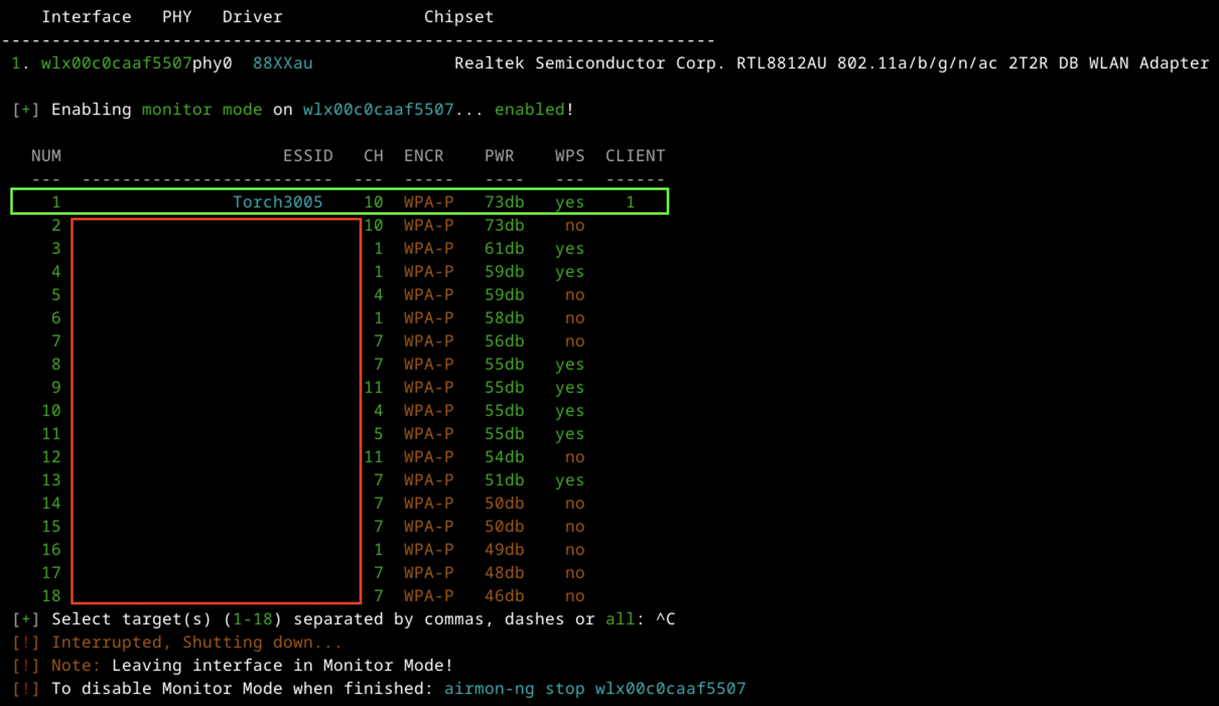
Let’s open GNU Radio Companion and create the new project.
By default, you have only 2 blocks: Options and Variable named “samp_rate”. We can keep Options as is, but “samp_rate” value let’s change into 2e7 (20 MHz).
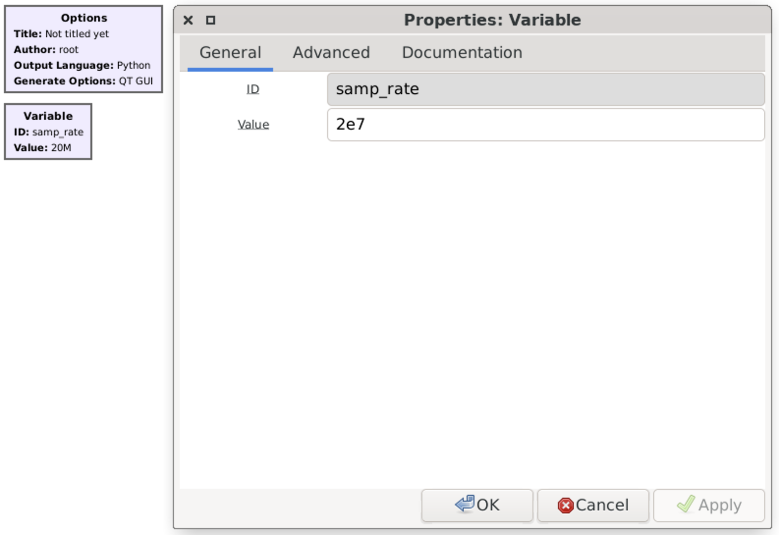
Next, let’s add another Variable, call it as “freq” and set up its value by frequency related to our home Wi-Fi channel – 2,457 GHz (2457e6).
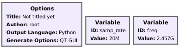
After that find “Noise source” block, add it to the chart and keep default values: Noise type – Gaussian, Amplitude – 1. Also add “Multiply const” and set it Constant value as 100 (that will be our amplifier).
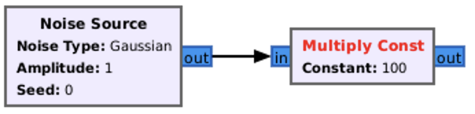
The last link in our chain is the transmitter by itself. Find “osmocom Sink” and add it to the chart.
We must change several values to make it work properly. First the “Sample Rate (sps)” must have “samp_rate” value.
Then, “Ch0: Frequency (Hz)” should be set up by our second Variable – “freq”.
RF, IF and BB Gain, based on our experience, could be 50, 20 and 20 respectively.
Finally, “Bandwidth” let’s set as 20 MHz (2e7).
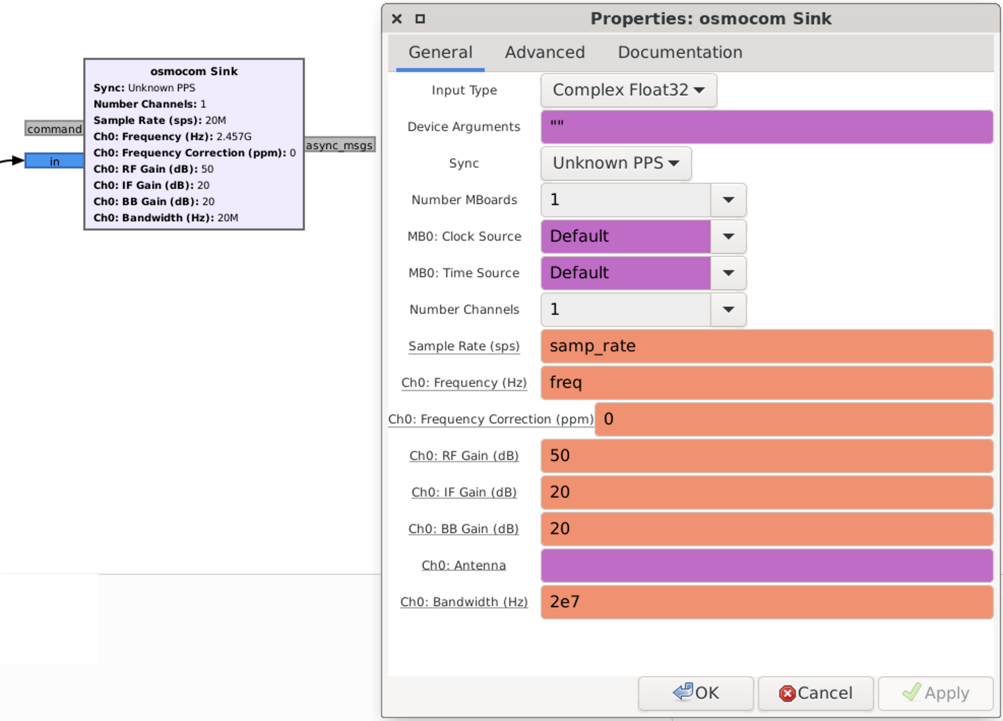
If you did everything correctly, you had to get the chart looks like that.
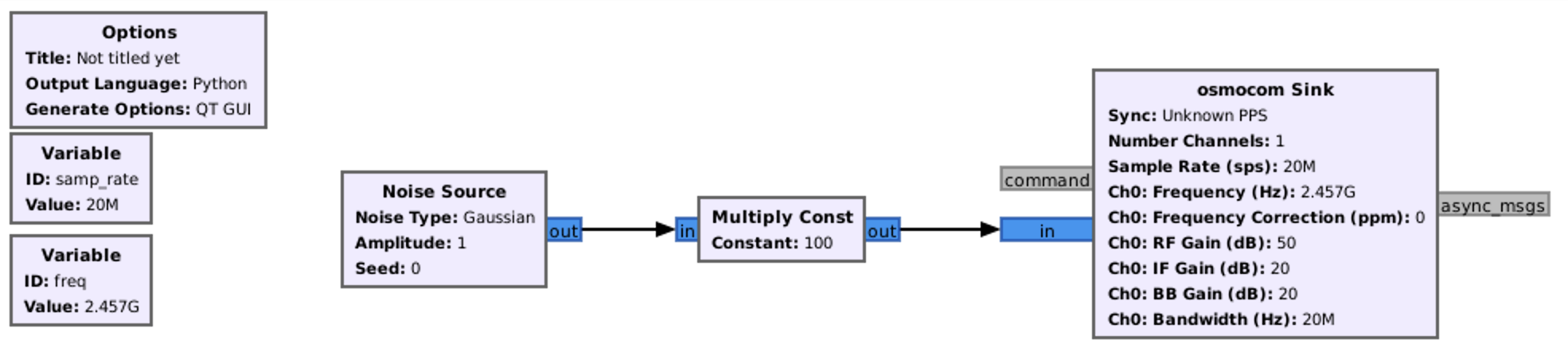
E. Voice broadcasting
Previously we talked about Walkie-Talkies and intercepting channel and, basically, we were just listening talks of other entities. Now, it’s time to have some fun and transmit some voice across the radio waves.
Before that, let’s agreed of some rules. As a frequency we will use 433.92 MHz as it’s legal in the country where we currently live; won’t be in the air for more than 30 seconds; nevertheless that HackRF transmit power is not high by itself we will use the power low enough just to transmit the signal over several meters.
The final graph is presented on the picture below and let us explain that in details to you.
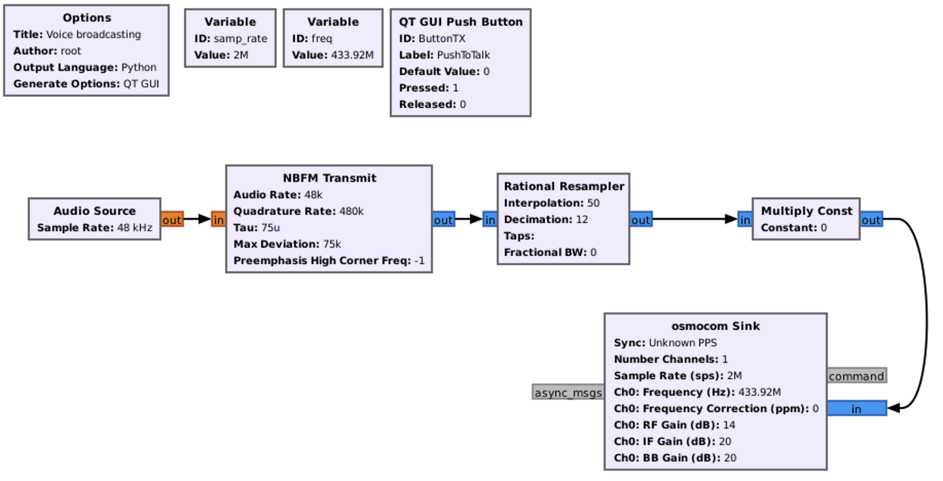
First, it’s “Audio Source” which is a block that provides audio data as the input to our signal processing flowgraph and used to capture audio from a microphone. The importance of setting up the audio source as 48 kHz for transmitting voice lies in the Nyquist theorem. According to the Nyquist theorem, the minimum sampling rate required to accurately capture a signal without losing information is twice the highest frequency present in the signal. By setting the audio source to 48 kHz, we ensure that the sampling rate is at least double the highest frequency in the speech signal, which means we can accurately capture the full range of audible frequencies in our voice.
Next is “NBFM Transmit” (Narrowband FM) which is a block used for transmitting a narrowband FM signal. Tau, Max Deviation and Preemphasis High Corner Freq values we will keep by default. But Audio Rate and Quadrature Rate we have to set it up as 48 and 480 KHz respectively. Why Audio rate should be 48 KHz we revealed in the previous paragraph. The rate of 480 kHz for Quadrature Rate is set to be ten times the audio rate. This choice ensures that the quadrature rate is significantly higher than the highest audio frequency. The higher quadrature rate allows for accurate representation of the frequency deviation needed for FM modulation, resulting in a faithful reproduction of the audio signal when transmitted.
The Rational Resampler is a block used for resampling signals (the process of changing the sampling rate of a signal, which can be necessary when interfacing different parts of a signal processing chain with different sampling rates or when adapting the signal to match a specific requirement). The Rational Resampler allows for both interpolation (increasing the sampling rate) and decimation (decreasing the sampling rate). The parameters that need to be set for the Rational Resampler are the interpolation and decimation rates. The interpolation factor specifies how much the sampling rate is increased, and the decimation factor specifies how much the sampling rate is reduced. Combining the interpolation factor of 50 and the decimation factor of 12 allows for converting the input signal to a different sampling rate while preserving the essential information in the signal. The interpolation ensures that the signal has enough samples to avoid loss of information during subsequent processing stages that may require a higher sampling rate. The decimation then reduces the number of samples to match the desired output rate without losing relevant signal content.
The next set of blocks is a combination of QT GUI Push Button and Multiply Const.
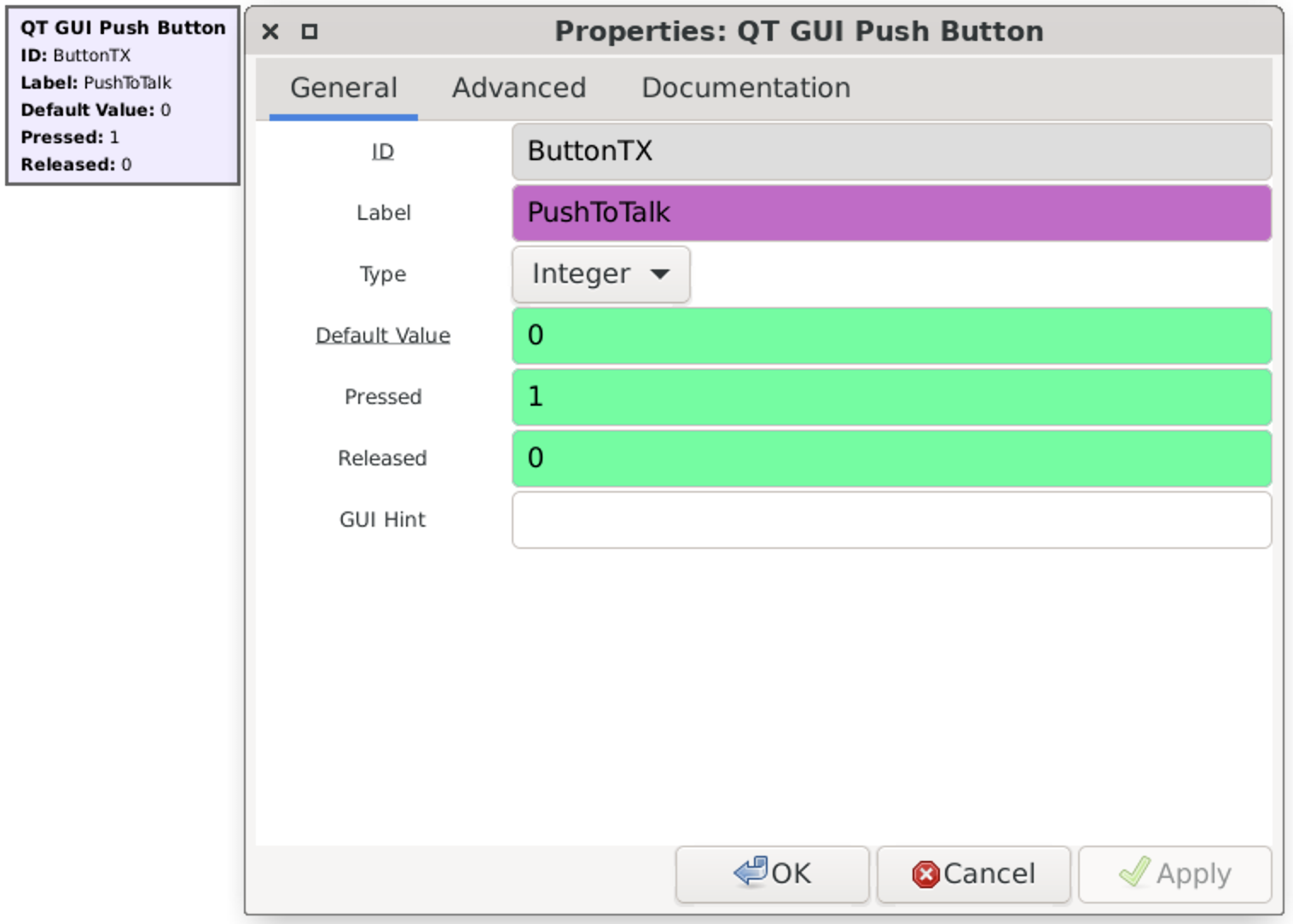
So, how the button is working. Default Value means the value after launching the application. Pressed and Released respectively the values when we click the button and release it.
The good news is that we can combine button’s value with other blocks, including Multiply Const. As a Constant value just put button’s ID hence each time we press the button the value becomes 1 and after releasing – 0.
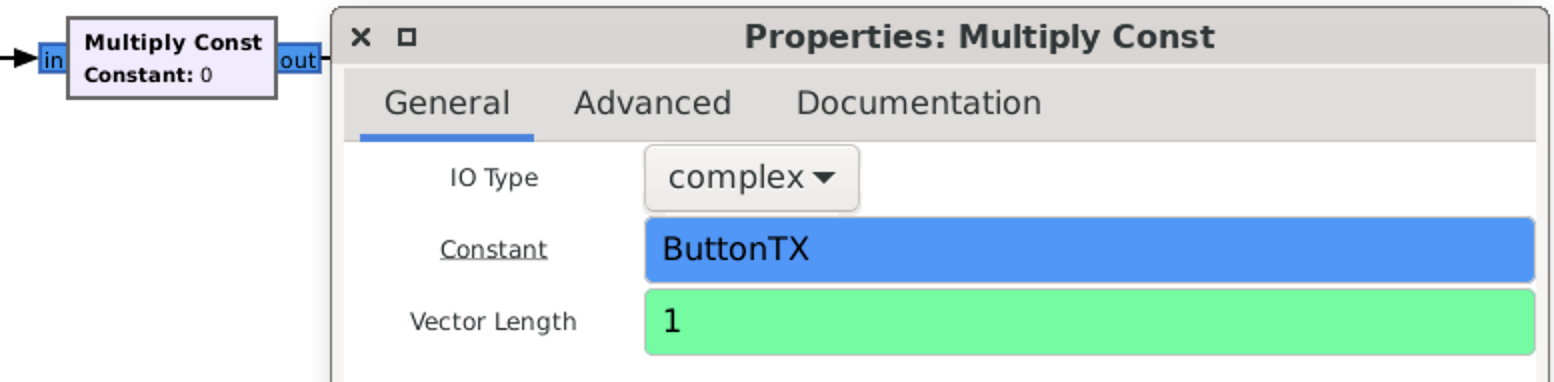
The last block is osmocom Sink which we discussed previously. Just don’t forget to set up a proper frequency.
If you followed the steps accurately, you should get a chart that appears like this.
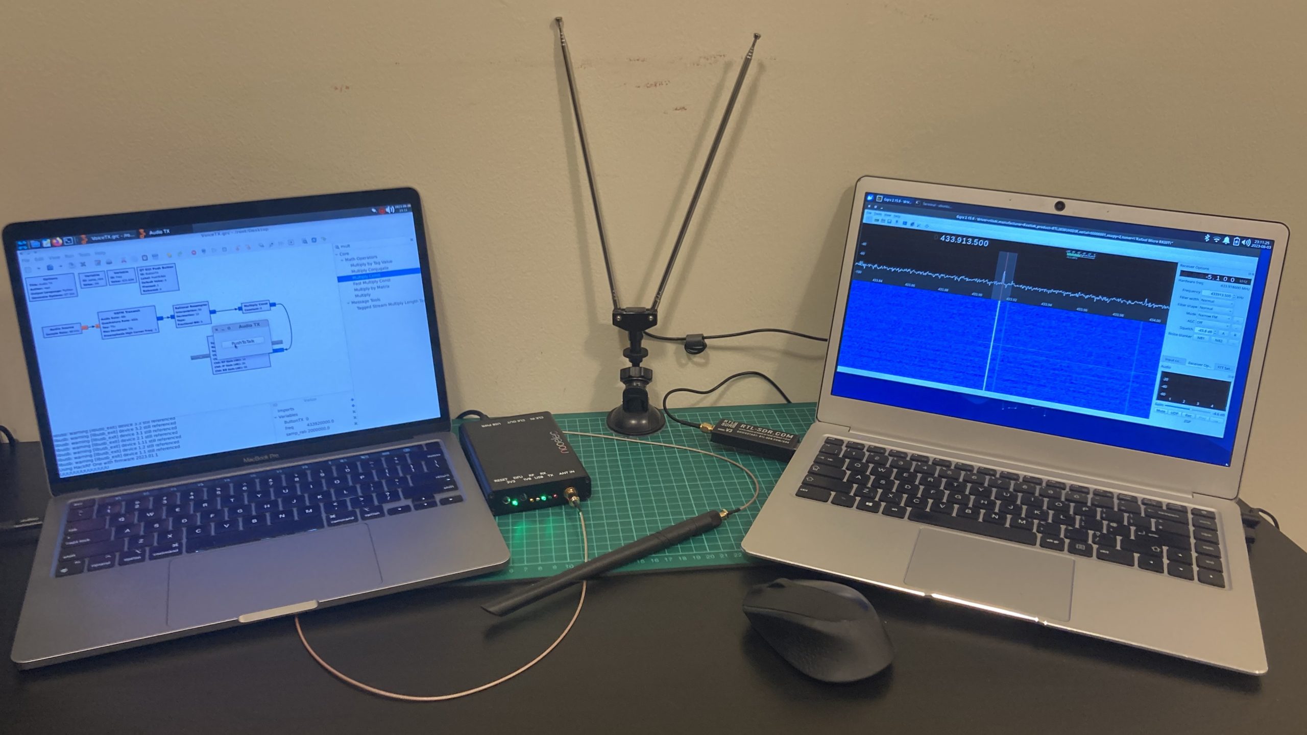
7. Hacking a doorbell
Let’s start our radio waves hacking journey with something easy and understandable. And wireless doorbell is the best teacher: it’s cheap, easy to install and with the permanent signal each time (not rolling code). Against a doorbell we can use replay attack as well as synthesized signal method to make it work.
Firstly, allow us to introduce you to our testing equipment – the Sky-Touch Wireless Doorbell. You can conveniently purchase it from online stores worldwide. This kit is priced at only 8.69 USD and includes two components: the doorbell unit itself and the accompanying button.
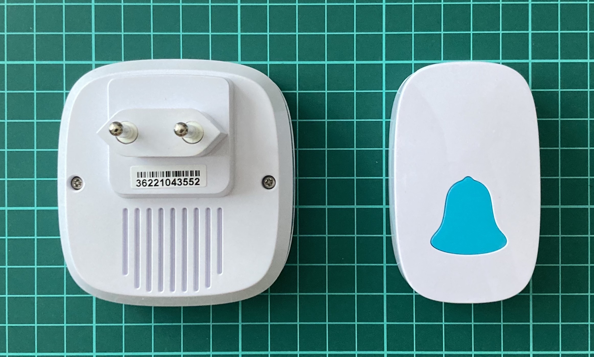
If you are going to order that please keep in mind the electrical plug is European type hence you have to purchase an adapter to your electrical supply in case you are living not in Europe.
Based on the User Manual the working frequency is 433.92 MHz ±0.5 KHz means from 433’919’500 till 433’920’500 Hz. That delta is not so much and we can ignore that, setting up the receiver and transmitter to 433.92 MHz, but for our research purposes we will definitely measure it.
One funny stuff regarding that kit is Wireless range: 300 meters (unobstructed). We have not measured that yet, but from our perspective and based on our experience it is a little bit exaggerated. Also, we can’t even imagine where you can use the doorbell 300 meters away.
Before going further let’s disassemble them and see how it’s inside.
A. Disassemble
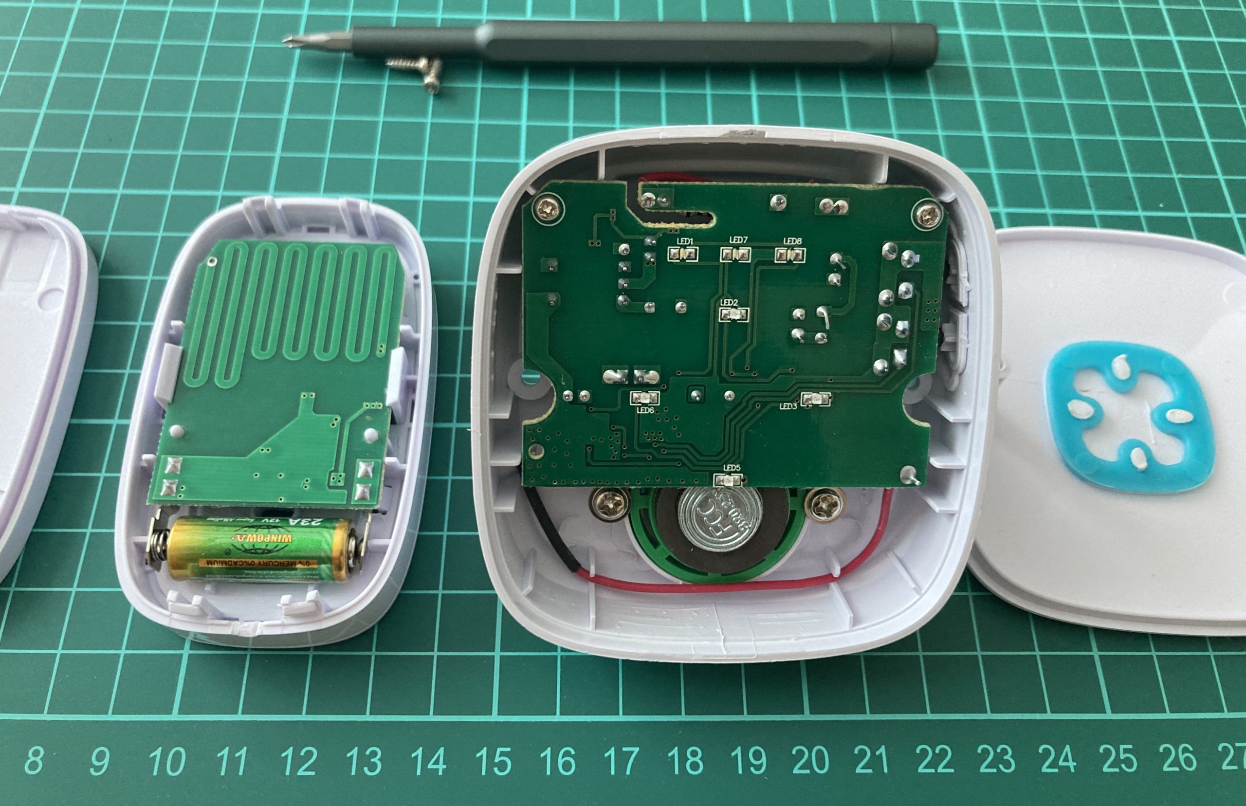
We will start from the transmitter – the button.
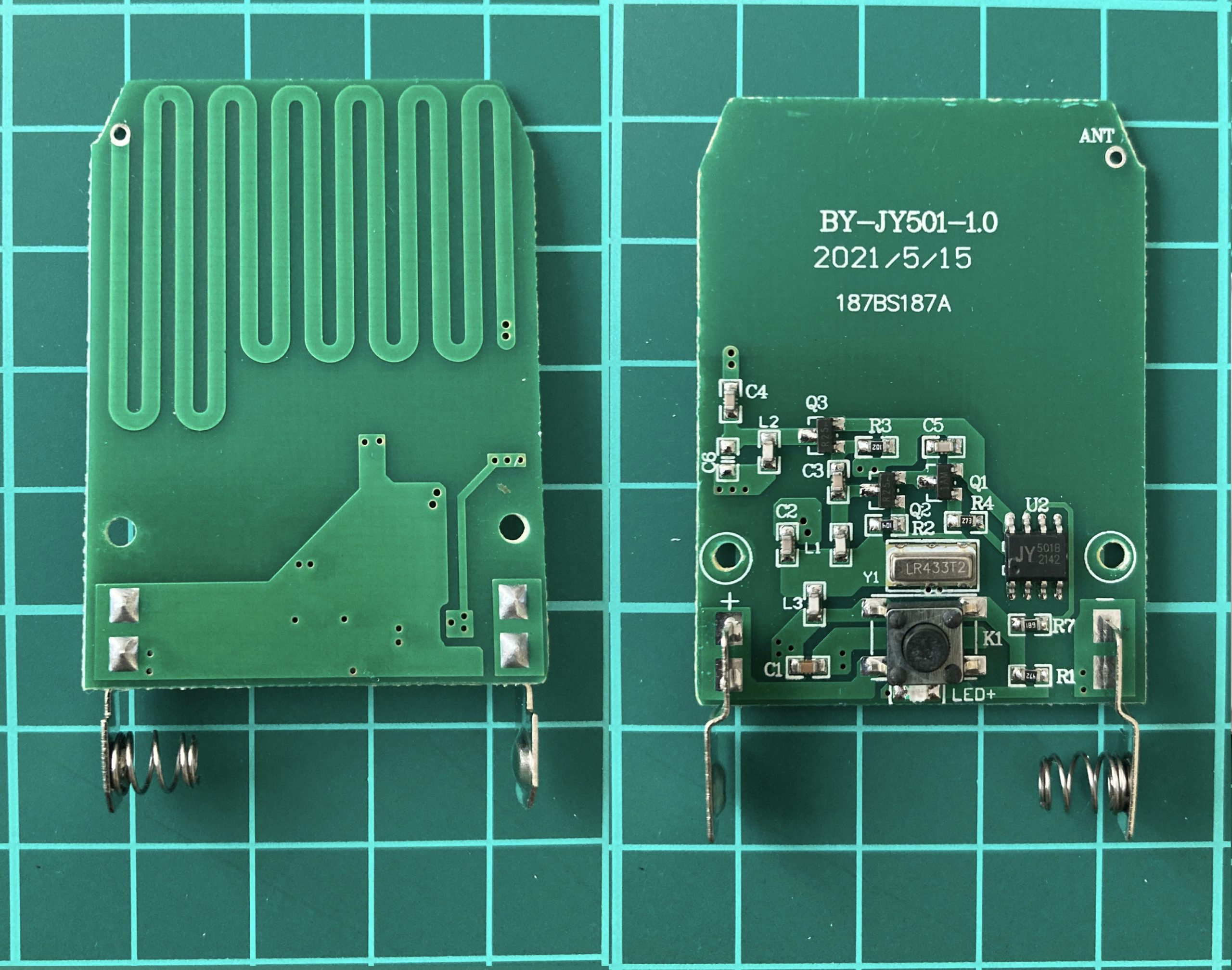
As you can mention, it’s quite straightforward. Except obvious contacts for a battery, there is a button to link the chain with a LED indicator next to it.
Next, the heart of the transmitter – the SAW (Surface Acoustic Wave) Resonator LR433T2. It is needed for frequency filtering and selection the 433MHz frequency range. The LR433T2 works by converting electrical signals into surface acoustic waves that propagate along a piezoelectric substrate. These waves undergo constructive interference at 433MHz, creating a resonant effect, allowing the LR433T2 to pass signals at its resonant frequency.
After that a chip JY 5018 2142 the main purpose of which is to generate the payload. Next, there are 3 transistors combined with capacitors and resistors to amplify the signal.
The last item is antenna which is made in a very interesting way – by PCB (Printed Circuit Board) trace. As you may remember from the chapter 4.B. the wave length for 433.92MHz is 69.1 cm. The trace length is roughly
31,6 cm (9 times of 2.3 cm, 3 times of 2.8 and 1 time of 2.5 cm) which is slightly shorter by 2.95 cm than the half-wave length.
What about the doorbell by itself?
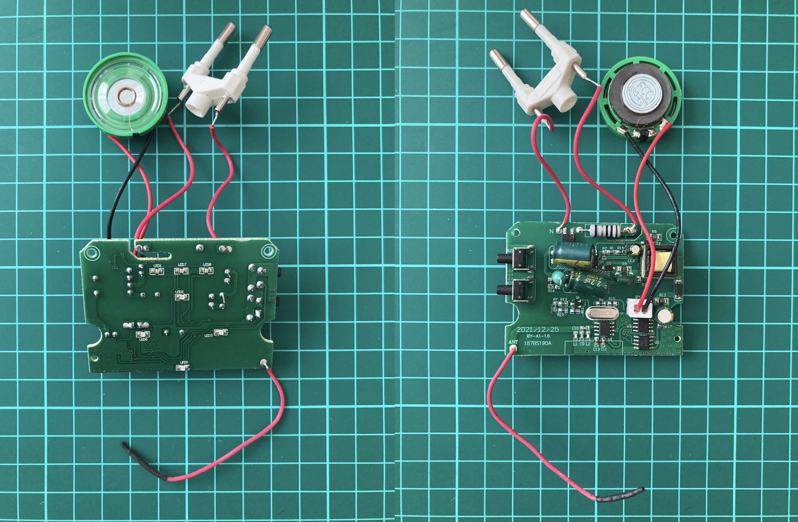
This scheme is a little bit more complicated comparing to the button one. Except the obvious electrical plug and the speaker, we can find 2 side buttons for volume and sound type adjustment, step down transformer, much bigger capacitors, our SAW friend and the 11.5 cm antenna (6 times of the wave length).
Now, when we know how it’s inside and high-level working approach, it’s time to assemble it back and perform the signal analyzing.
B. Defining the frequency
Based on the User manual as well as SAW Resonator LR433T2, we assume that the working frequency for our wireless doorbell is 433,92 MHz. We trust but let’s check it to be 100% sure.
To do that we will use 3 different applications: CubicSDR, GQRX and Universal Radio Hacker.
Let’s start from CubicSDR. Set the central frequency up to 433.92 MHZ with 0.5 MHz delta and launch it. During the capturing let’s press the doorbell button and see the peak.
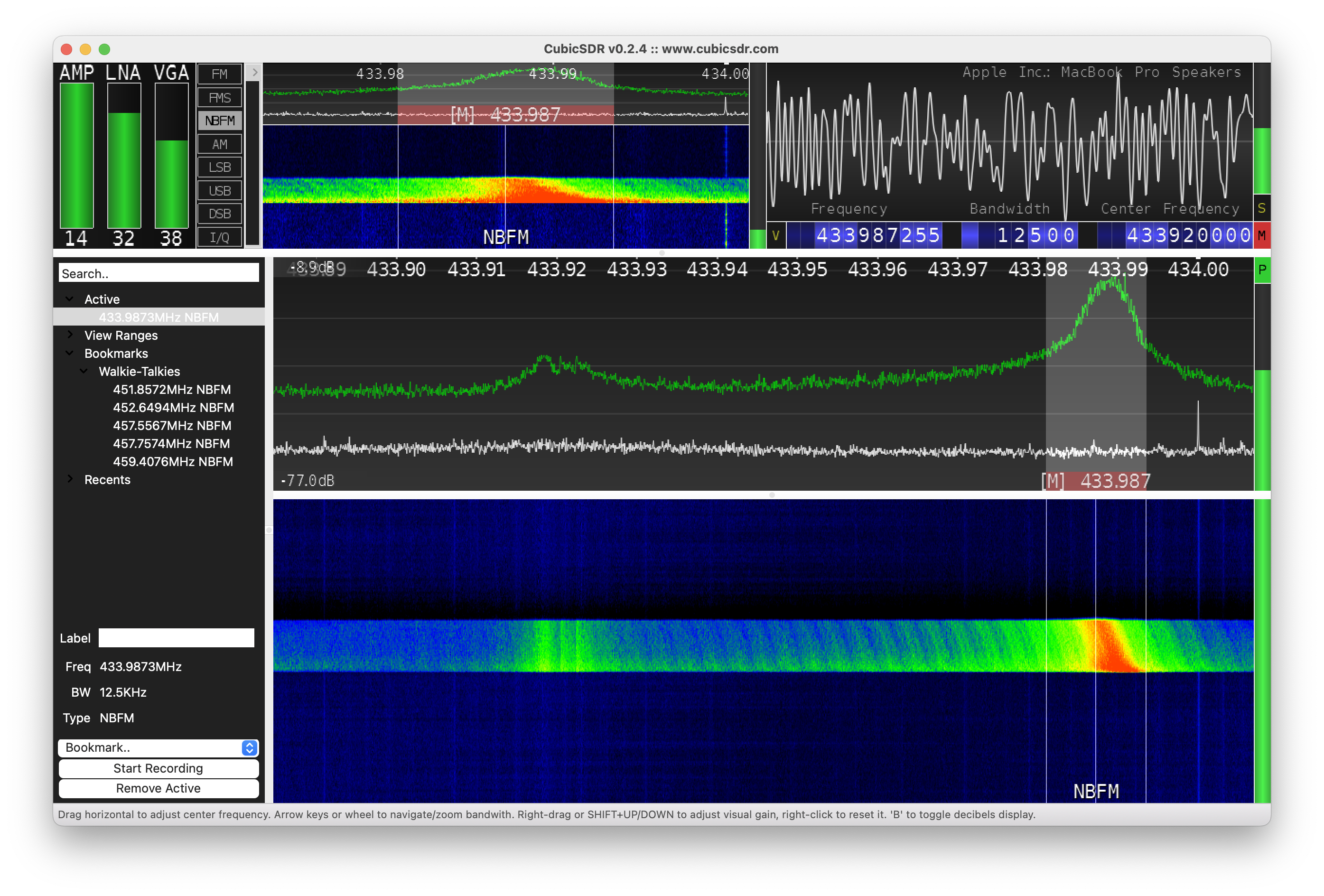
Hm, don’t you think it’s a little bit strange, that the frequency is 433.987 MHz instead of 433.92 MHz, even with the delta of 0.5 KHz?
Ok, let’s check another application, maybe there is a CubicSDR misunderstanding. Let’s launch GQRX.
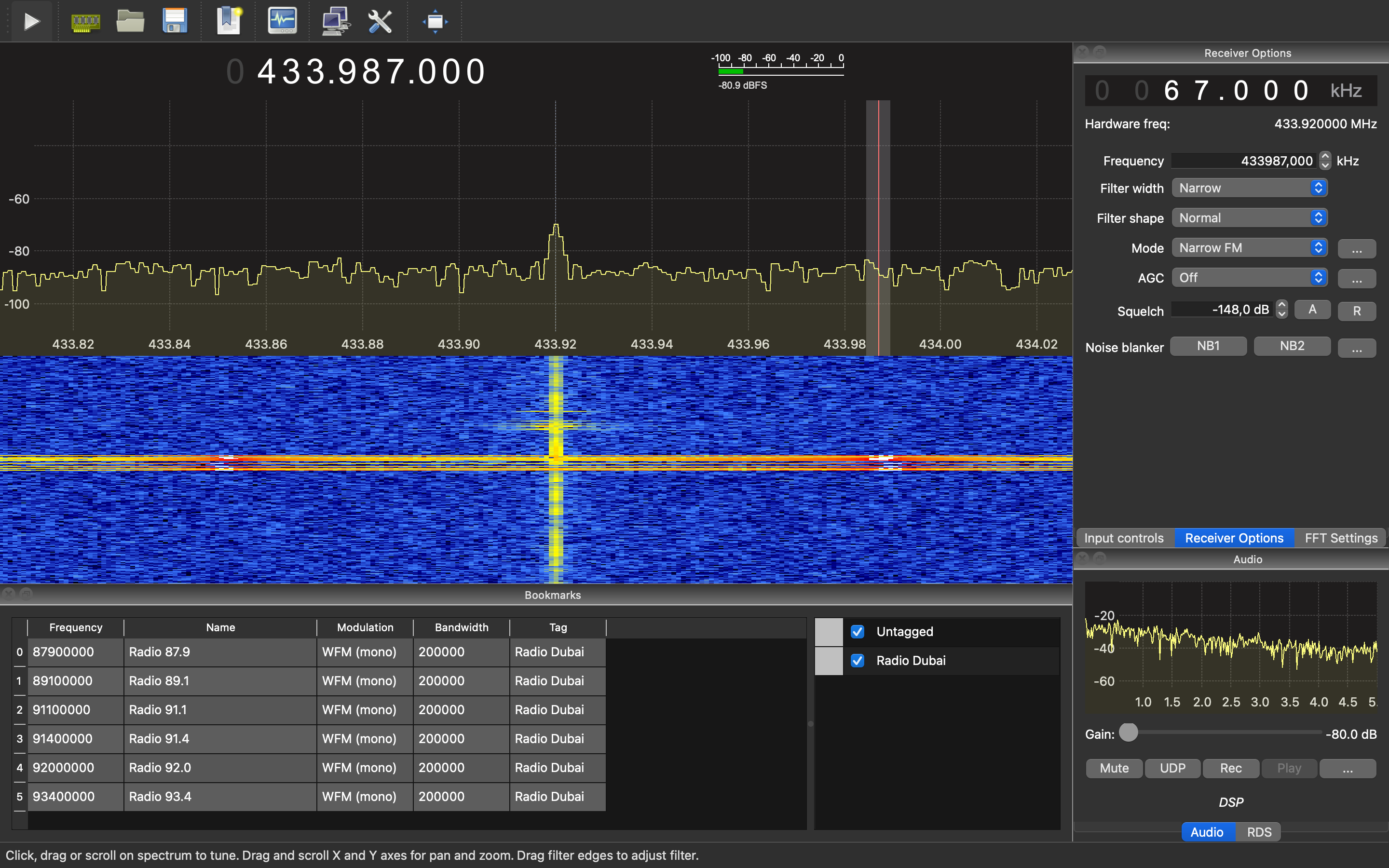
Once again, it’s 433.987 MHz. Let’s check once again, but using URH app.
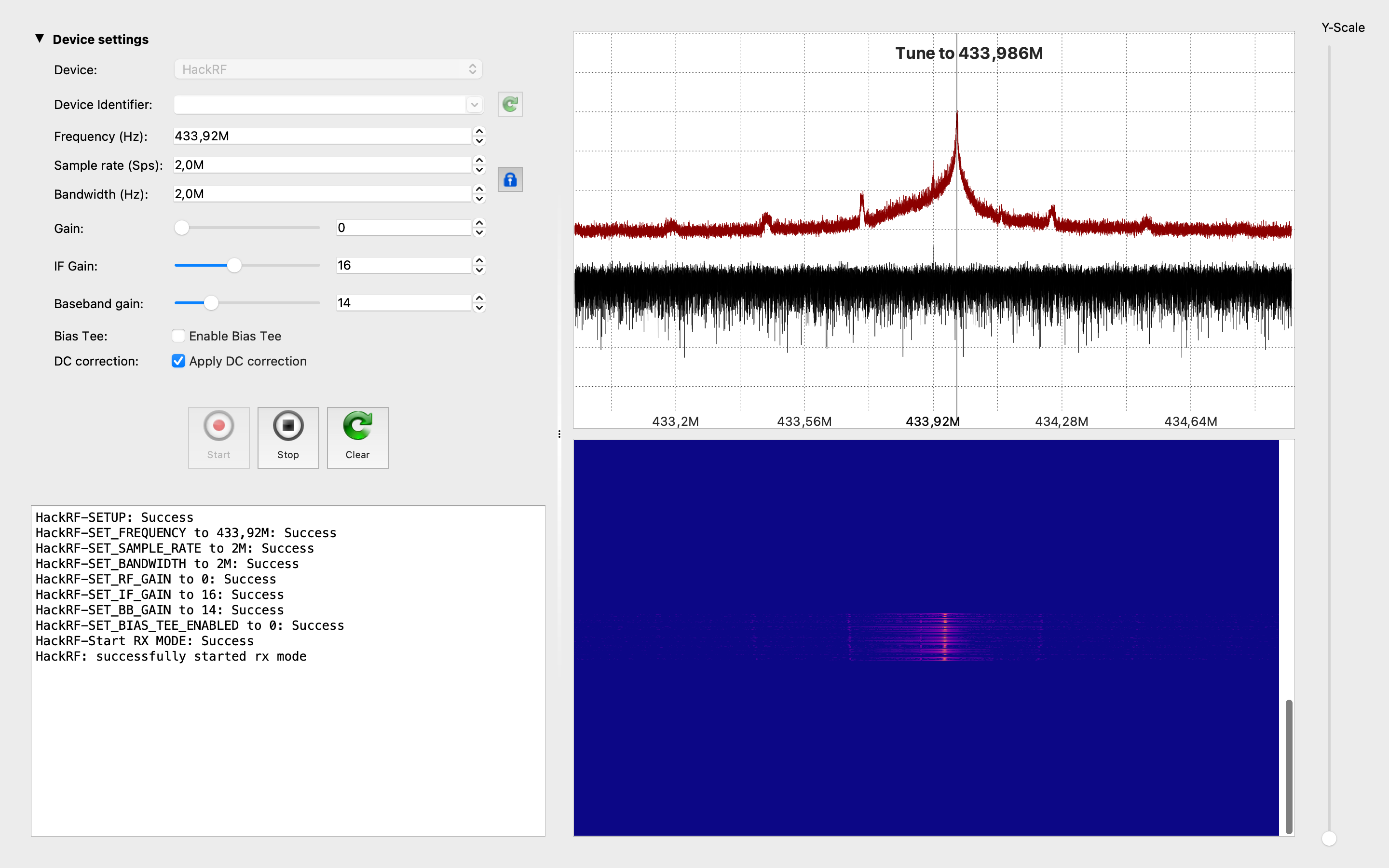
That’s weird: three different applications showed 433.987 MHz for the equipment supposed to work on 433.92 MHz.
To be sure it was not HackRF’s fault we did the same measurements with RTL-SDR dongle (but with different antenna) and the results were almost the same – 433.981 MHz.
Why does it happen this way, and what are the underlying causes?
There are several possible reasons why wireless stuff overall is operating at a slightly different frequency than the specified one. Some of the root causes for this discrepancy could be:
- Manufacturing Tolerances: The components used in the stuff’s circuitry, such as crystals, capacitors, and inductors, have manufacturing tolerances. These tolerances can cause slight variations in the frequency of the circuitry, leading to a different operating frequency than intended.
- Aging and Environmental Factors: Over time, electronic components can age, which may cause changes in their characteristics, including frequency. Environmental factors such as temperature, humidity, and exposure to external interference can also influence the circuit’s performance and result in frequency drift.
- Design Fluctuations: The stuff’s design might have incorporated certain factors that affect the frequency, such as variations in the physical dimensions of the circuit board or the antenna.
- Frequency Calibration: During the manufacturing process, the stuff’s frequency might not have been precisely calibrated to 433.92 MHz, leading to the observed frequency difference.
- Interference: The stuff might be affected by nearby electronic devices or radiofrequency interference, causing the circuit to resonate at a different frequency.
- Firmware or Software Issues: In some cases, the stuff’s firmware or software might be programmed to operate at a different frequency due to an error in programming or settings.
- Counterfeit or Non-Standard Components: If the stuff uses components that are not genuine or deviate from standard specifications, it may result in unexpected frequency behavior.
- Manufacturing Variations: If the stuff is produced by different manufacturers or production batches, there might be slight variations in the circuitry that lead to frequency differences.
What is the real cause in our particular situation we can only guess, but basically it does not matter till the doorbell is working and we know the real transmit frequency. Moreover, let’s keep in mind that it is the button’s frequency: the button is sending signals on that range. But do we know the real and exact frequency the doorbell by itself is receiving signals? Unfortunately no and it’s a real challenge to do that. Nevertheless, let’s stick with 433,98 as the transmit freq.
C. Replay attack
Let’s start our hacking with the easiest one exercise – replay attack. But what a replay attack is and how it’s working?
A replay attack, also known as a replay assault, is a type of cyber attack that targets wireless communication systems and involves capturing and later retransmitting valid data packets to impersonate a legitimate user or device.
Here’s how a radio waves replay attack typically works:
- Data Capture: The attacker uses specialized hardware or software to intercept and capture the radio frequency signals transmitted between two legitimate parties (for example, between a wireless sensor and a control system).
- Data Replay: After capturing the data packets, the attacker stores them for later use. The captured packets contain essential information, such as authentication credentials, control commands, or any other sensitive data that may be used for malicious purposes.
- Replay Attack: Later, the attacker resends the captured data packets back into the communication channel. Since the data packets are valid and were previously captured from a legitimate communication session, the system receiving the packets may perceive them as coming from a genuine source and act accordingly.
The impact of a successful radio waves replay attack can vary depending on the system being targeted. In some cases, it could lead to unauthorized access to a secure network, manipulation of control commands, impersonation of legitimate users, or the extraction of sensitive information.
Speaking of the doorbell – the impact is low… except if you want to prank your neighbor, but even in that case he/she can just unplug it as a protecting approach.
Less words and more actions. Let’s directly dig into it.
C.A. hackrf_transfer
The first replay attack approach in our list is using default HackRF apps – hackrf_transfer (we discussed about it in 2.A.B. section of this article/book).
Before collecting the signal and transmit it back, let’s find out what keys of the app is crucial to our attack:
- -r <filename>: save the data into file (we will use it during the capturing phase)
- -t <filename>: transmit data from file (we will use it during the attack by itself)
- -f <freq_hz>: frequency in Hz
- -s <sample_rate_hz>: sample rate in Hz
- -x <gain_db>: TX VGA (IF) gain (how powerful is the transmitter)
Ok, let’s combine it all together and write the receiving command:
hackrf_transfer -f 433987000 -s 2000000 -r doorbell
and transmitting command as well:
hackrf_transfer -f 433987000 -s 2000000 -t doorbell -x 45
Once again:
- -f 433987000: the working frequency, in our case it’s 433.987 MHz
- -s 2000000: the sample rate, in our case it’s 2 MHz
- -r/-t doorbell: write/read the file, in our case it’s “doorbell”
- -x 45: transmit power, in our case it’s 45 dB
If you did everything correctly, you have to receive and save the signal and then transmit it back – the doorbell should ring.
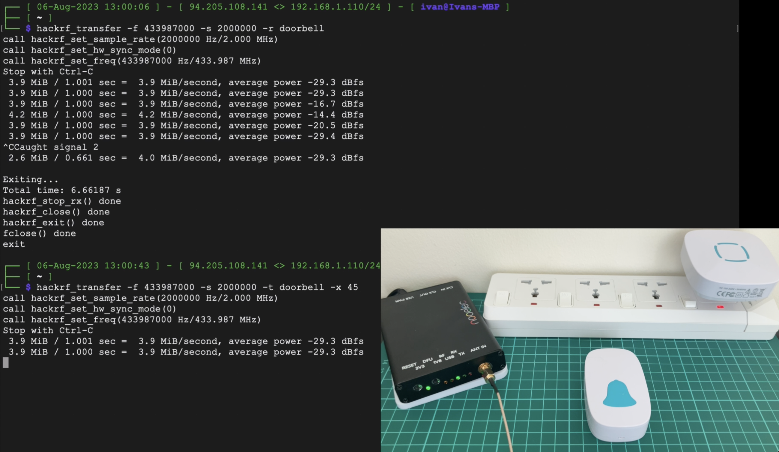
C.B. Universal Radio Hacker
Next in our replay attack applications list is URH. To be honest, if you don’t want to figure out how everything is working, you are afraid of the command line and just wanna click one button “Make me happy” – it’s your application On the other hand, if you are guru knowing almost everything and just want to automate your routine work or perform really fast – URH is one of the best solutions as well.
Ok, let’s launch that and select “Record signal” from the “File” of the main menu. The new opened window has several presets, which we have to set:
- Device: select “HackRF”
- Device Identifier: just click the refresh button. But if you have only one connected HackRF no need to do that (but we do)
- Frequency (Hz): by default it’s been set as 433,92M. We may keep that freq, but it’s better to put 433,987
- Sample rate (Sps): by default it’s been set as 10,0M. Let’s adjust it as 2,0M
Basically, in that particular situation with a doorbell, all you need to mandatory change is the Device. But we are learning and have to do everything correctly despite the final result.
Having done all the settings, just press the “Start” button.
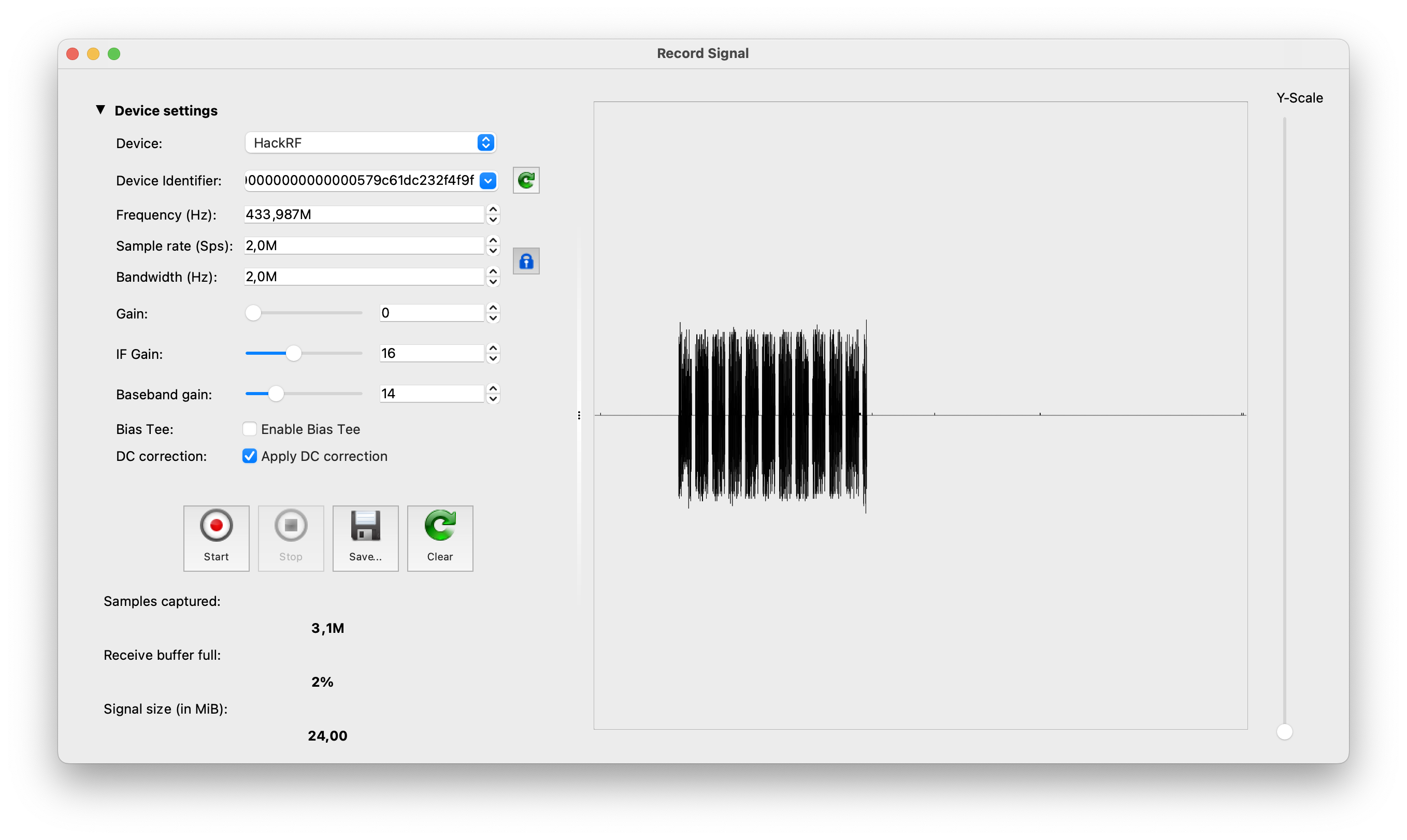
Once you captured the signal, press the “Stop” button and then “Save” it. After that just close that window and the application will automatically open the new one with the replay feature.
All that you have to do is just click the “Replay signal” button and hear the doorbell.
All that you hac to do is just click the “Replay signal” button and hear the doorbell.
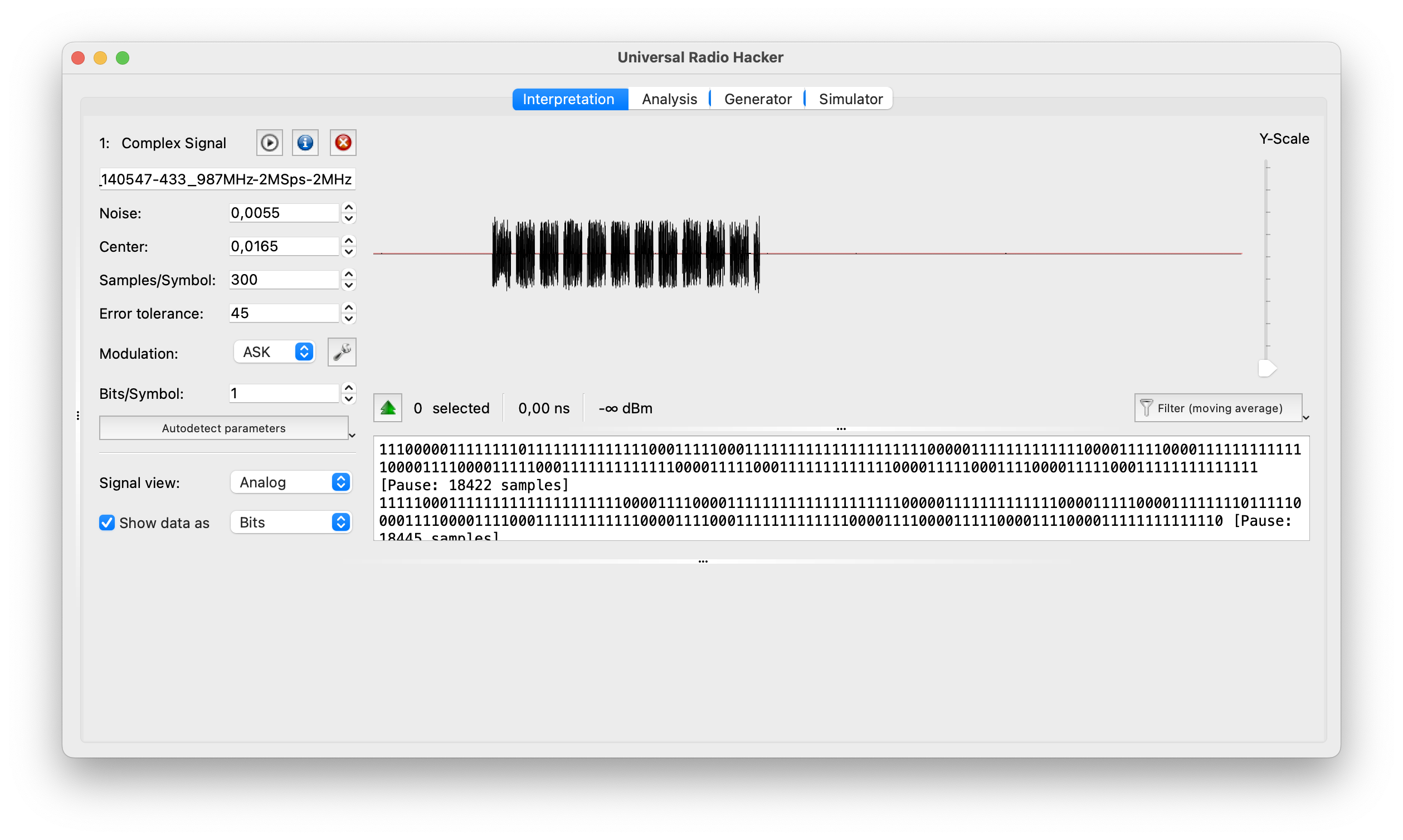
C.C. GNU Radio Companion
And the last, but not the least in our list is GNU Radio Companion. Perform a replay attack using that app is a little bit more complicated, but still manageable.
To perform the replay attack we need 2 graphs: the first one is for receiving the signal and the second one is for sending the payload.
Let’s start with variables which will be the same for both graphs: Sample rate as 2 MHz and the Frequency as 433.92 MHz (for this time let’s keep it 433.92 instead of 433.987 MHz).
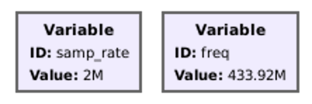
Basically, for receiver and transmitter we need only 2 main blocks: “osmocom Source” and “File Sink” for receiver and “File Source” and “osmocom Sink” for transmitter. But for the visual approvement everything is working fine we added “QT GUI Time Sink”.
Osmocom Source and Sink settings you can find on the following screenshot. The file with a payload is named “doorbell” and stored in the Desktop directory. Don’t forget to set it up as well.
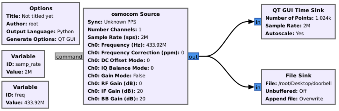
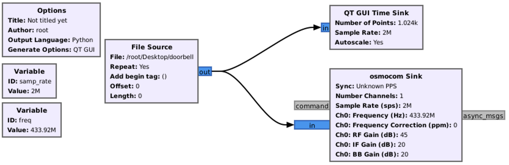
So, first we have to launch the receiver graph and during its working time save the signal. After that stop the graph and launch the transmitter graph. If you did everything correctly you would listen the doorbell’s ring.
D. Getting the payload
Ok, the replay attack is the great feature if you want to save a time and the signal is permanent and not changing (rolling code). But knowing what is under the hood, how it’s working and, based on your knowledge, synthesize the exact same signal with payload is the real kick. Let’s tore apart the doorbell signal and synthesize back.
D.A. Universal Radio Hacker
We will start with our old friend – URH. So, once again, capture the signal like we did in 7.C.B., save it and keep it’s opened on the analyzing page.

So, the window is divided into 3 parts:
- The left one with some settings (keep it as is so far)
- The right top with the analog signal
- The right bottom with the code demodulator
As we can see the signal is quite clean and accurate that even the demodulator is showing the same values each time which is quite rare.
First, what we can do, but it’s not necessary in that particular case, remove the blank signal. You can do it either selecting the payload and “Crop the selection” or select the blank and “Delete selection”. We prefer the first approach as its less efforts consuming.
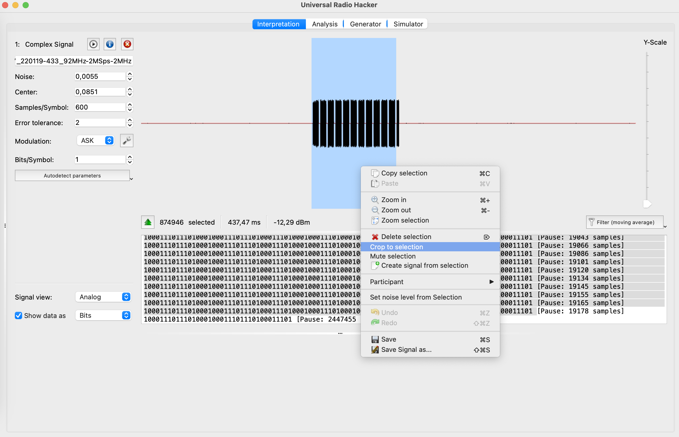
After that we get only the payload without any blanks.
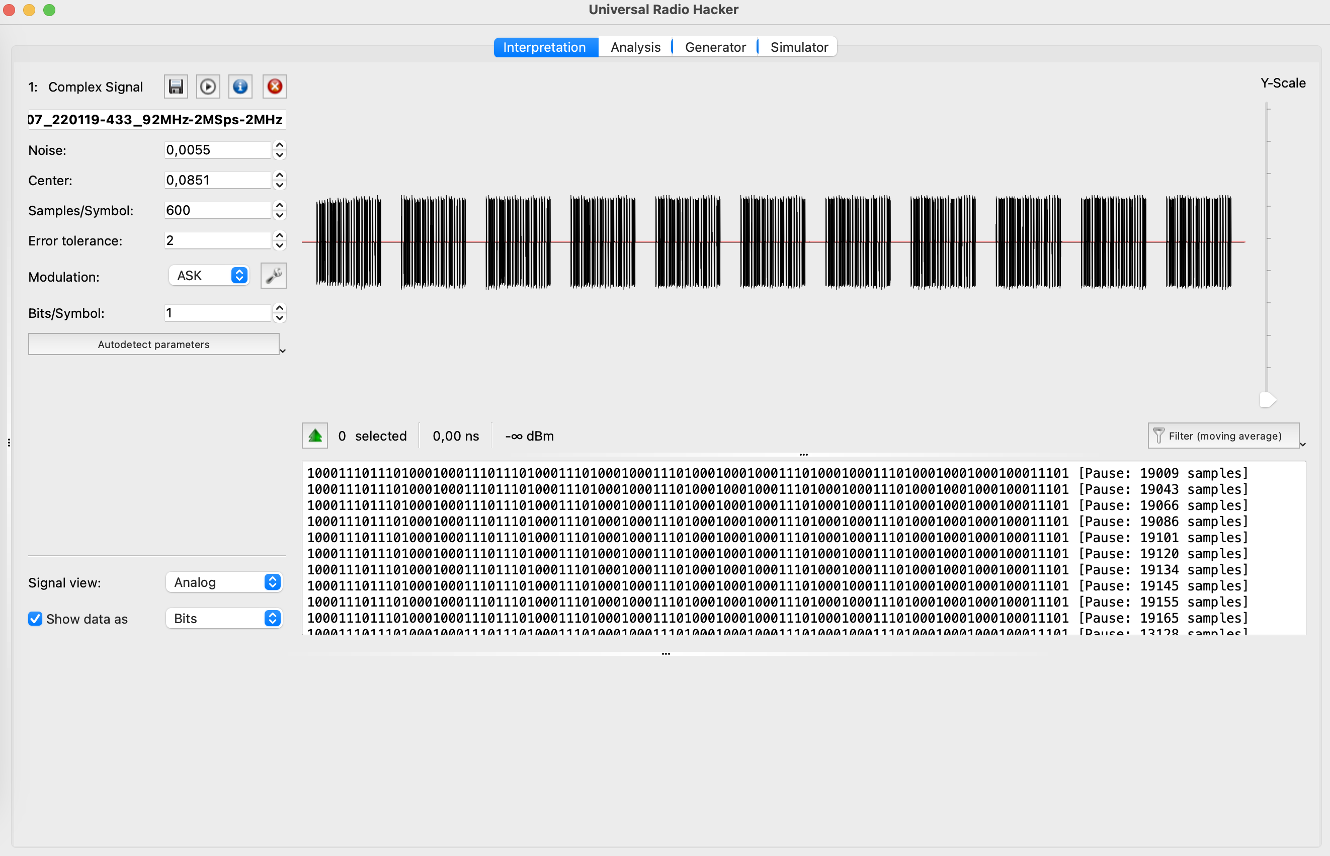
Next, let’s zoom it in. What can you tell us about the signal? First, it’s repeatable, means each time it’s sending the same payload (not the rolling code). In that case we can only consider one bunch of payloads rather than all of them.
Also, even right now we can create a pattern for that signal. Let’s consider that the short ones are 0 (zeros), and long ones are 1 (ones). In that case we can already get the payload as 0110011010010001001000010.
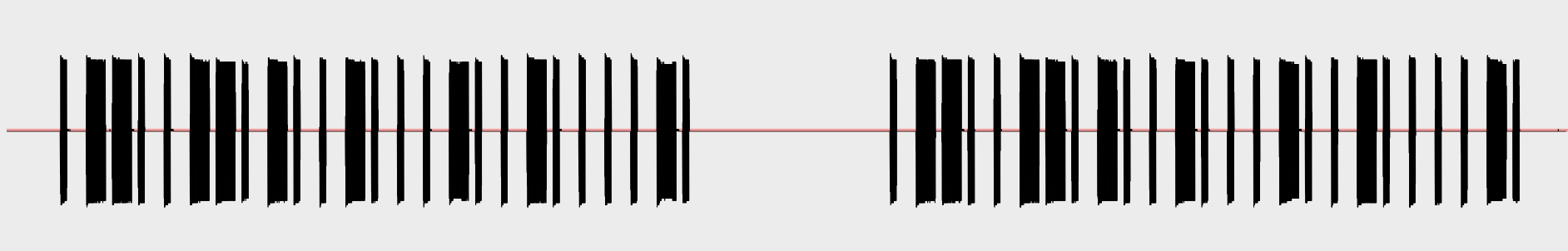
But, let’s do some more magic and amend some settings. As the “Signal view” (left bottom settings) choose the “Demodulated”.
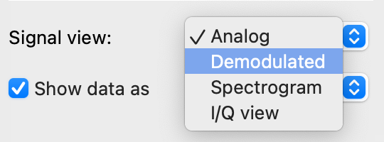
And now let’s look at the graph.
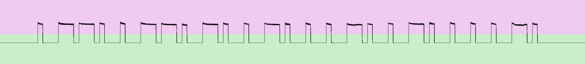
Wow, after the demodulation the signal became so clear and neat. That is the exact payload that the doorbell button is sending and the doorbell by itself has to receive to ring.
The only one question you may ask is why we defined the payload as 0110011010010001001000010, but the application is showing us the 1000111011101000100011101110100011101000100011101000100010001110100010001110100010001000100011101.
Let’s explain that. We defined the payload logically: we can see the short peak and say it’s 0, we can see the long one – 1. But the application has another approach: if the signal is up – 1, if the signal is down – 0.
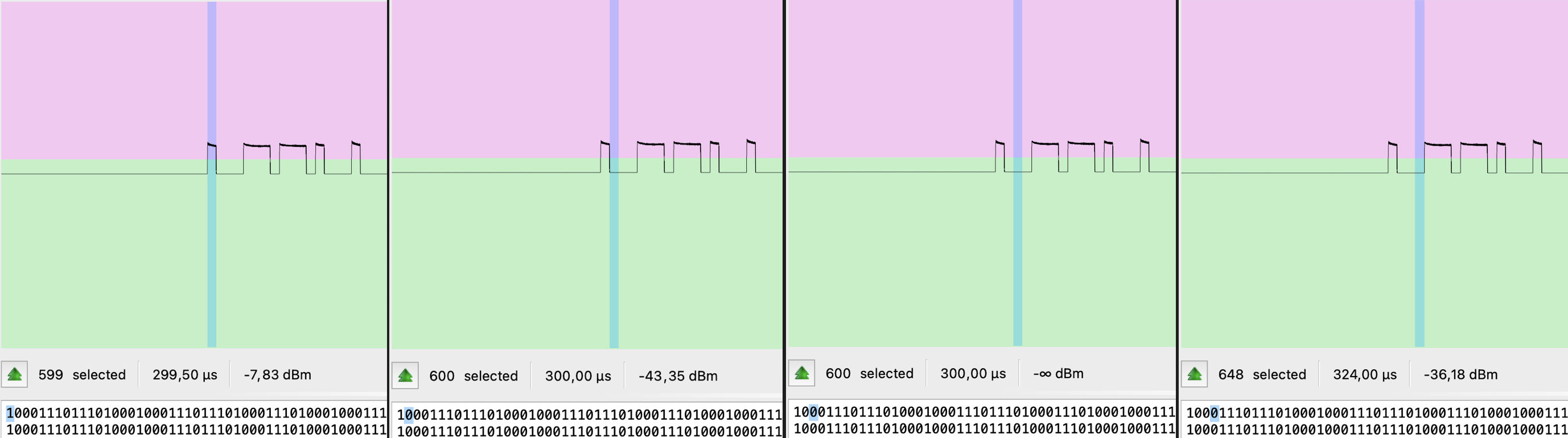
One more crucial moment we have to discuss. As you can see each part of the signal consists of 4 (four) items (25% each). For 0 (zeros) it’s 1000, for 1 (ones) it’s 1110. That aspect is mandatory. Just keep that in mind but we will come back to it during the synthesizing.
D.B. Inspectrum
Next application we want you to deal with is inspectrum. It has another workflow, maybe a little bit tricky, but still quite useful and understandable.
First, we need to record a signal within another application (unfortunately, inspectrum does not have that kind of feature) – for instance, GNU Radio.
As always, 2 variables: “Sample rate” as 2 MHz and “Frequency” as 433.92 MHz. “Osmocom Source” and “File sink” are mandatory to get the signal and save it, but we would also suggest including “QT GUI Time Sink” to see if it’s working. The last mandatory block is “Complex to Mag^2” which is used to calculate the squared magnitude of a complex-valued signal. This block takes a complex input signal (consisting of both real and imaginary components) and produces an output signal that represents the squared magnitude of the input signal.
The scheme should be something like that:
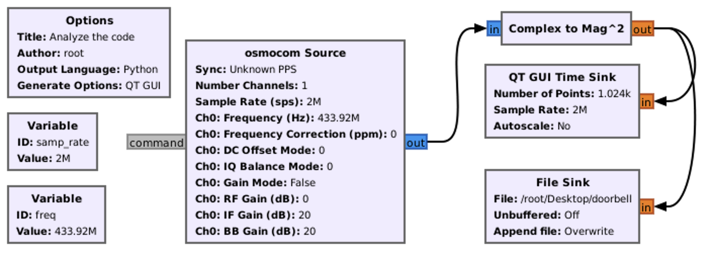
After executing the graph and saving the file, open inspectrum application and load the doorbell saved file. The result can shock you
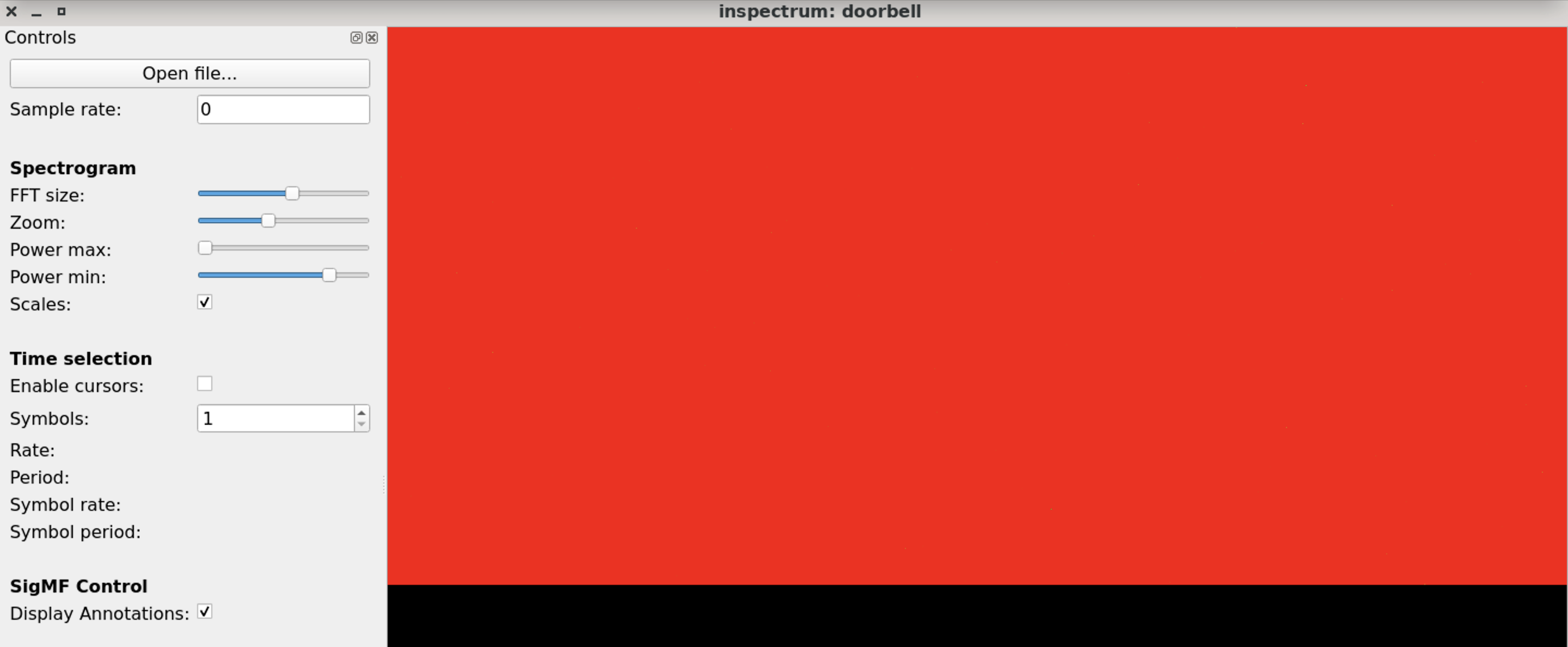
It’s a little bit surprising from the first look due to it’s all red or something. But, once you perform some setting adjustments, set up the sample rate and switch on cursors – that app will be your favorite.
First, let’s play with “Power max” and “Power min” ranges. Amending them you can find the payload.
Next, set up a “Sample rate” with the value we used to save that – 2000000.
After that check the “Enable cursor” checkbox and calculate the whole signal with the pause.
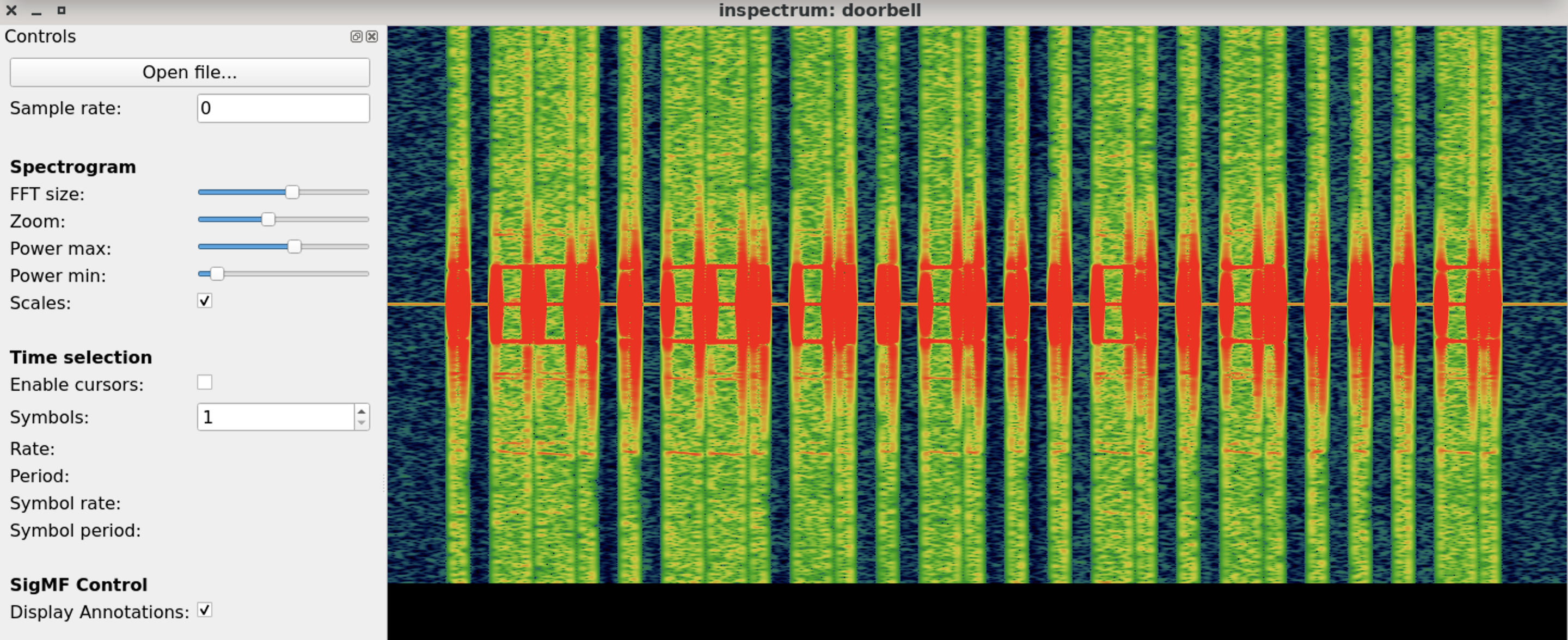
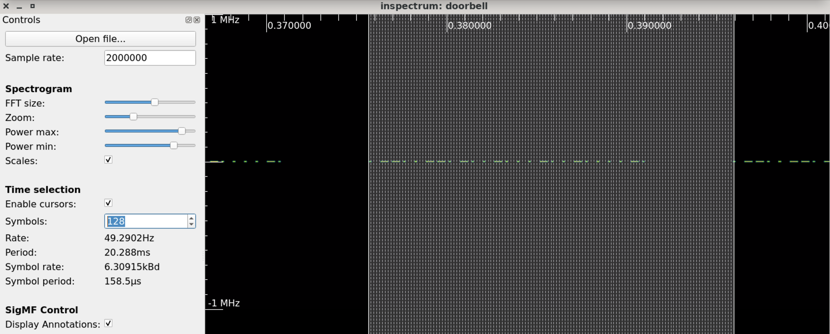
Or, if we calculate each line as a solid signal, not divided into 4 parts.
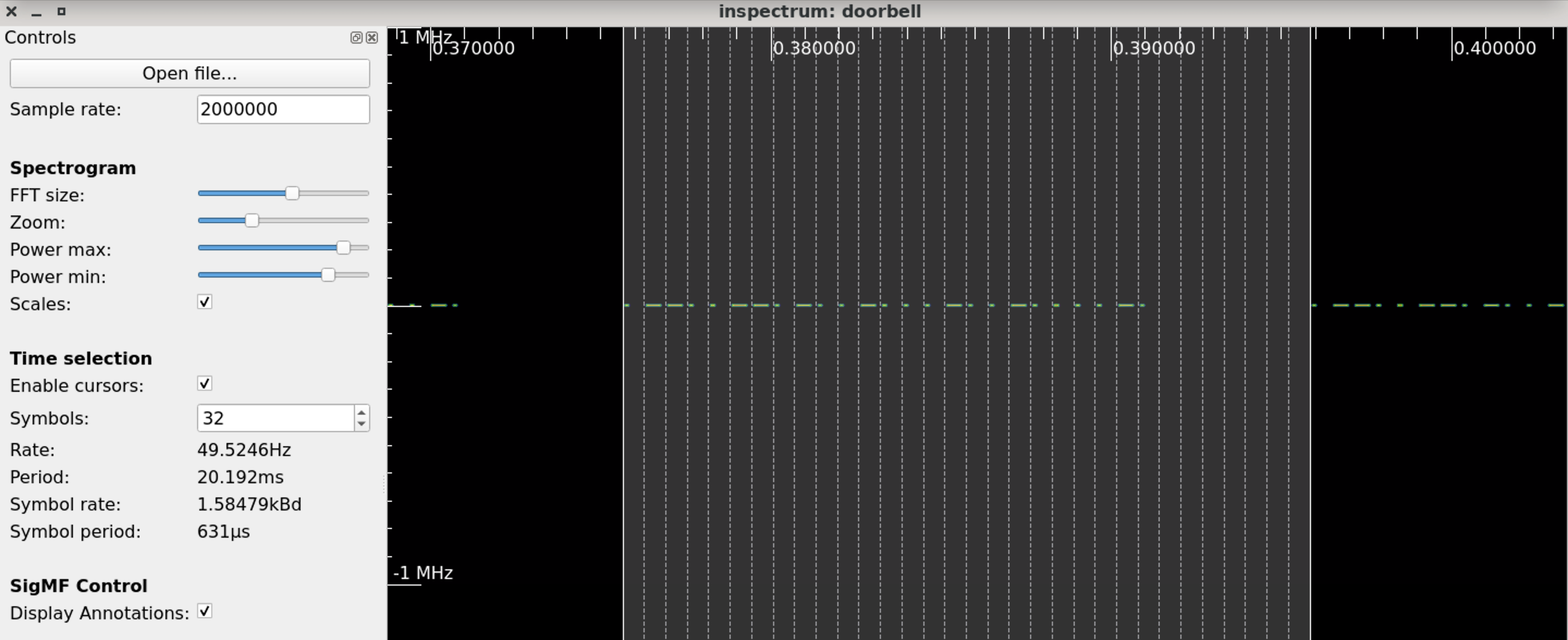
As you can see, the app requires more sensitive settings, but the result is awesome.
As you can see, we had the same payload, surprisingly (we are joking) – 0110011010010001001000010, which means both methods are working well.
D.C. Audacity
The last in our list of analyzing the signal is Audacity – the common audio editor on Linux. But besides working with audio files, the app can handle radio waves snapshots as well.
Let’s use the audio file from the previous paragraph and open it within Audacity.
First, we have to import the file as a “Raw Data”.
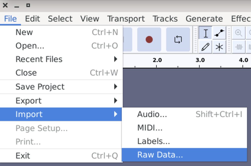
Once you choose the file, select settings as:
- Encoding: 32-bit float
- Byte order: Little-endian
- Channels: 1 Channel (Mono)
If you did everything correct, the graph should appear.
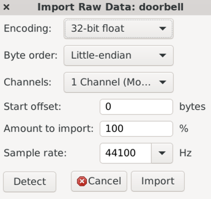
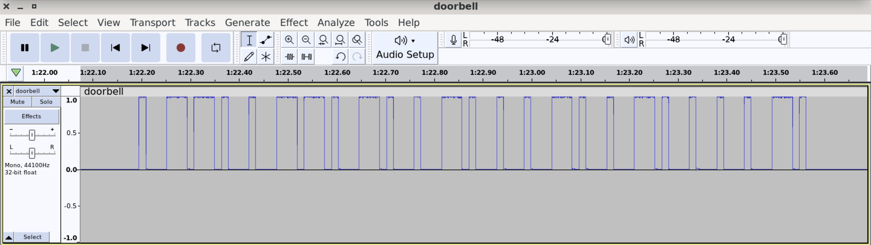
Overall, as you can see, it does not matter what application to use. It’s all based on what you personally prefer and convenience to use. So, choose your instrument and start analyzing.
E. Easy synthesizing
So, what we’ve done? We defined the frequency – ~433,92 (433,987 MHz), we caught the signal, analyzed it and got the payload. The next and logical step is to generate aka, using the wide-spread definition, synthesize the signal with the payload so the doorbell can ring without touching the button. Having said that, let’s do it.
As a main tool we will use GNU Radio Companion hence launch the application and create a new project.
Like we did it previously, let’s start with 2 variables: Sample rate as 2 MHz and the Frequency as 433.92 MHz.
Now, find and add the new block called “Vector Source”. The “Vector Source” block is a fundamental source block used to generate a sequence of complex numbers, forming a vector, that serves as the input signal for our signal processing flowgraph. This block allows us to manually define the values of the complex vector, which can represent a variety of signals or data.
The vector is putting in brackets, divided by comma format – (0, 0, 0). In our case, using the simple format of 1000111011101000100011101110100011101000100011101000100010001110100010001110100010001000100011101000, plus the pause between signals of 0000000000000000000000000000 (7 times for 4 items), the vector will be the next:
(1,0,0,0,1,1,1,0,1,1,1,0,1,0,0,0,1,0,0,0,1,1,1,0,1,1,1,0,1,0,0,0,1,1,1,0,1,0,0,0,1,0,0,0,1,1,1,0,1,0,0,0,1,0,0,0,1,0,0,0,1,1,1,0,1,0,0,0,1,0,0,0,1,1,1,0,1,0,0,0,1,0,0,0,1,0,0,0,1,0,0,0,1,1,1,0,1,0,0,0,0,0,0,0,0,0,0,0,0,0,0,0,0,0,0,0,0,0,0,0,0,0,0,0,0)
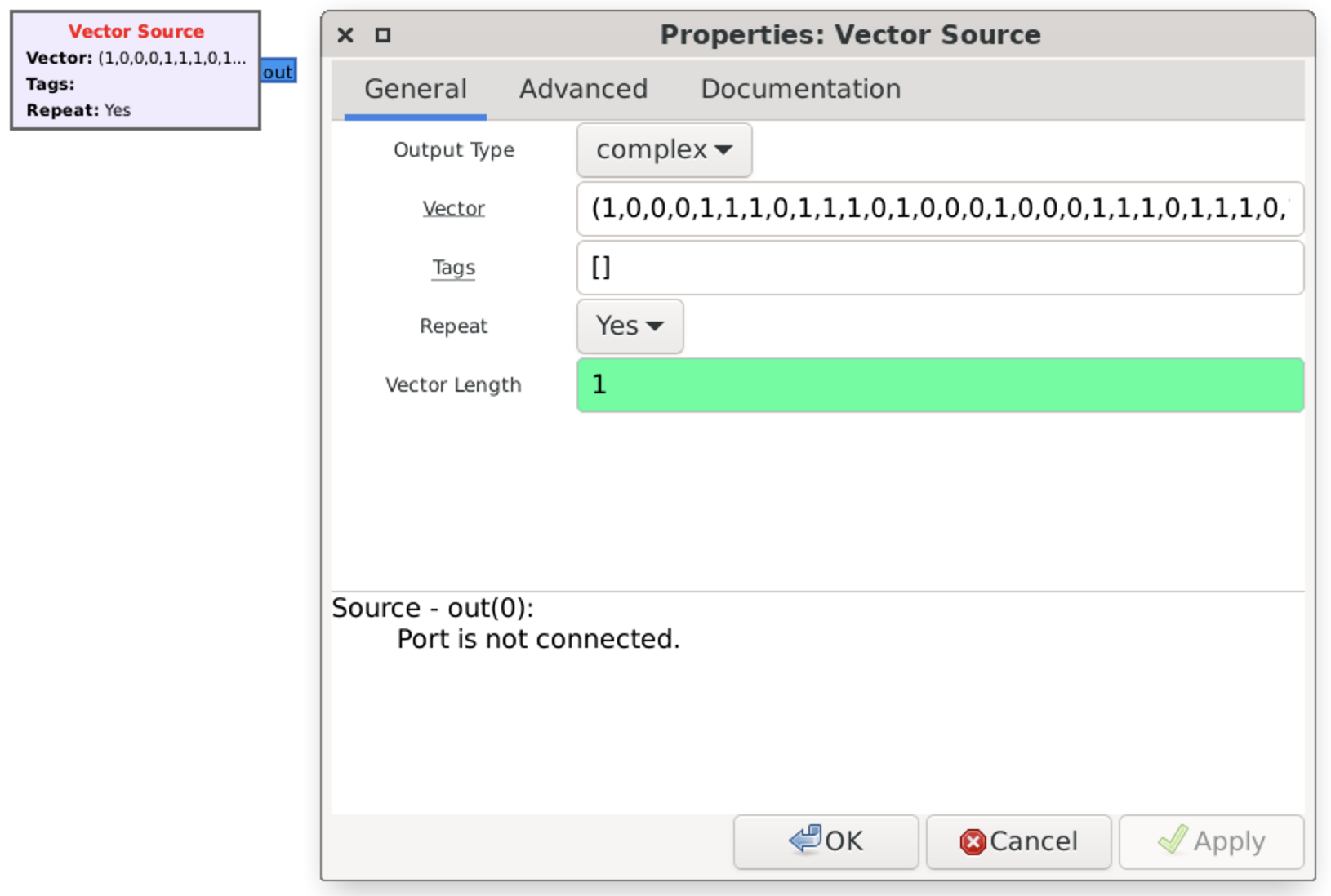
Next, we have to connect it with another block called “Repeat” (number of times to repeat the input, acting as the interpolation factor). Why do we need it? Basically, each payload, each peak and even each pause has a duration. Hence, to generate the correct payload we have to know the duration of the signal and implement that into our scheme.
To do that, open Audacity and import our previously recorded file. Zoom it in so you can correctly select the shortest peak. At the “Selection” menu set “Start and Length of the Selection” and see the output.
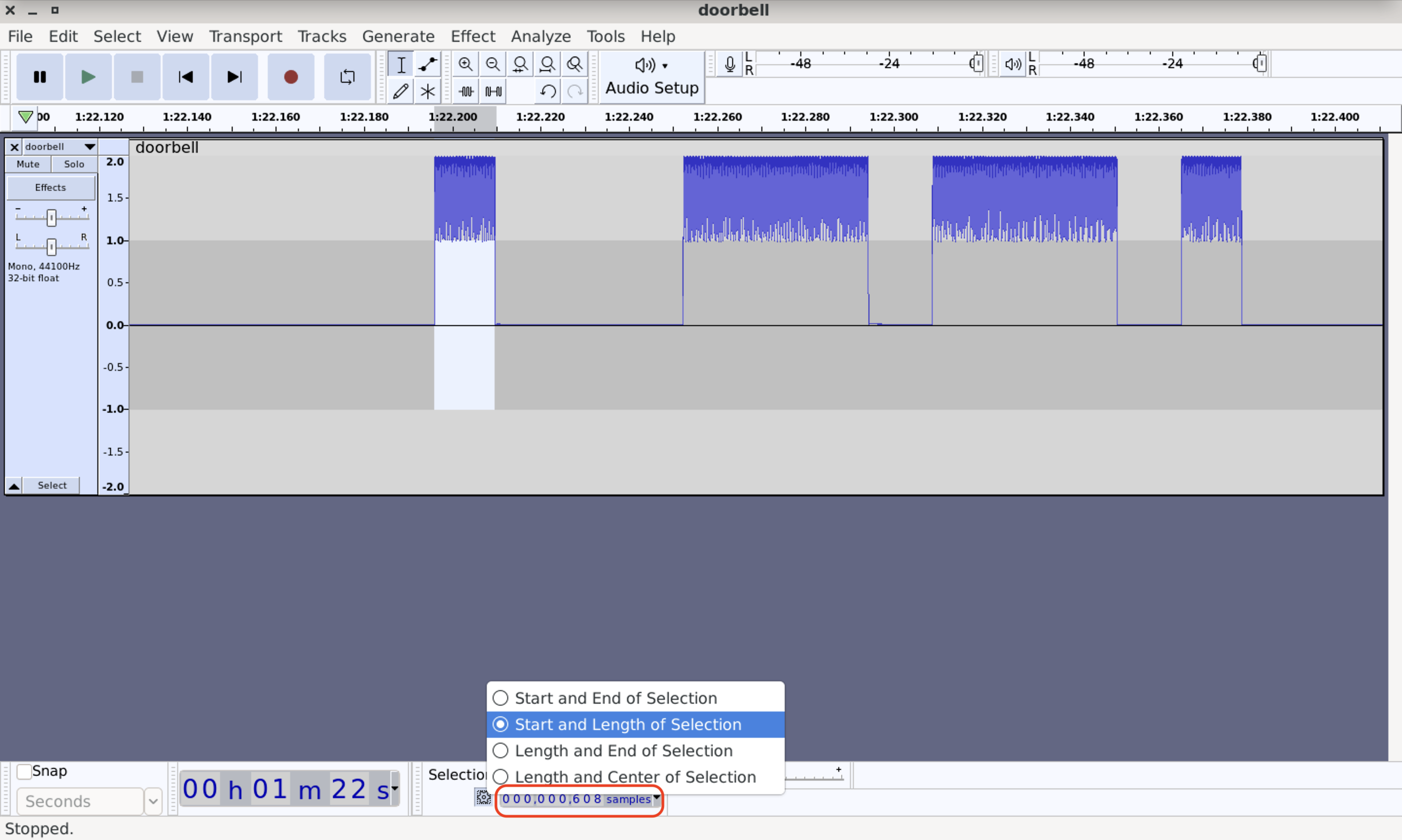
In our case there are 608 samples which we should put into our Repeat block.
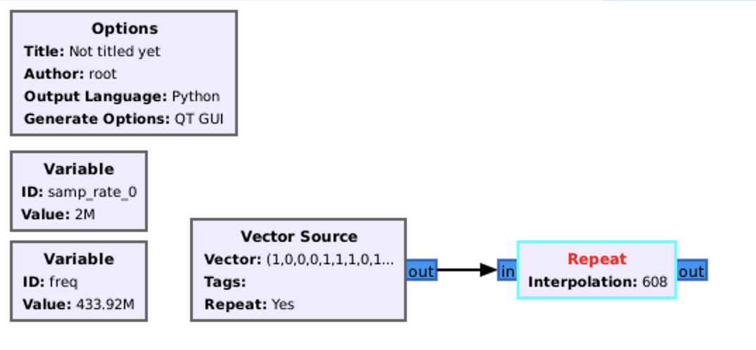
Just to check, that everything is working well, let’s add our old friend “QT GUI Time sink” and launch the script.
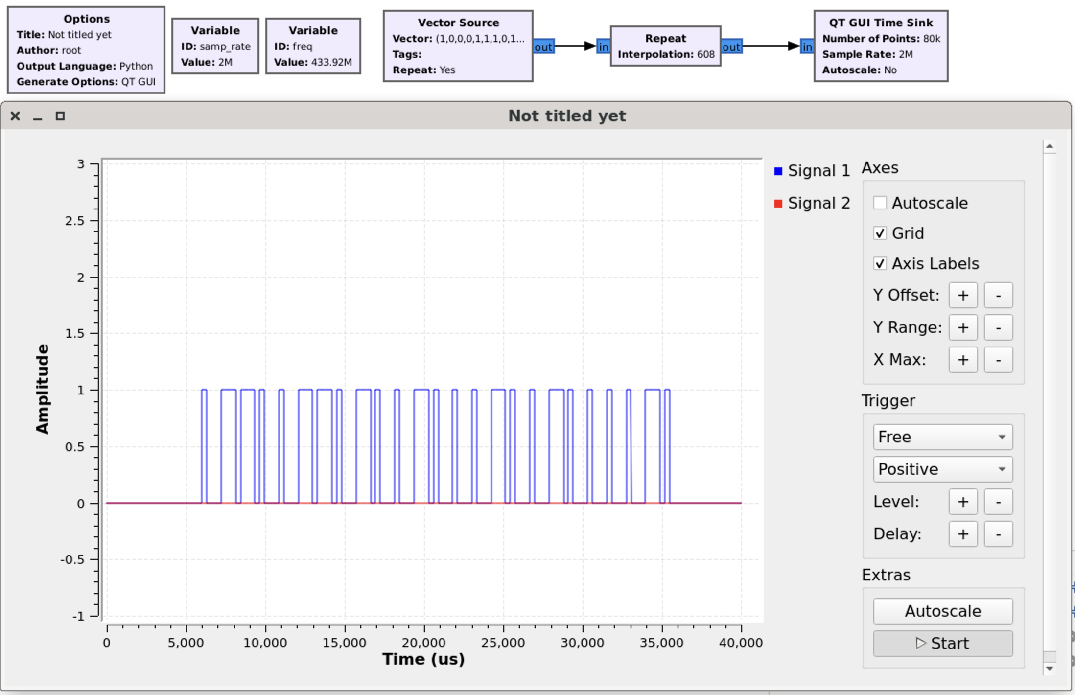
Great, guess all is working well. All we have to do is to implement the transmitter and the button, which is optional. But for our perfectionism soul it’s important 🙂
So, the final scheme is the next.
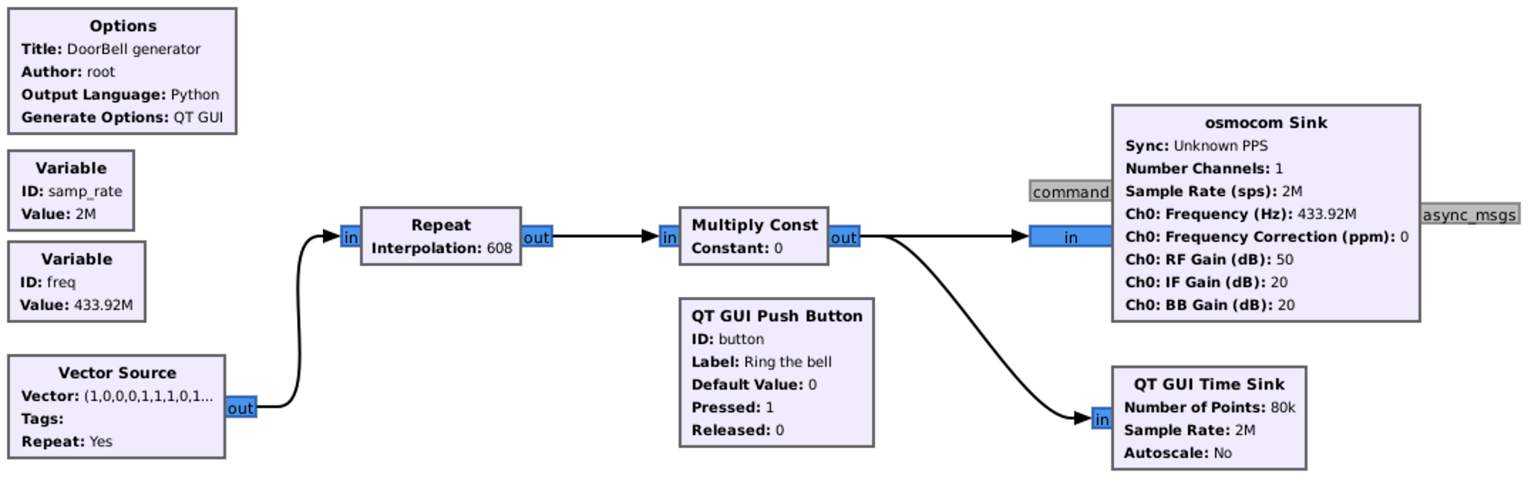
F. Smart synthesizing
Great, we synthesized the signal and the doorbell rang. And the flowgraph is quite easy and understandable. What and why should we do more if it’s working?
The answer is that for the long-term hacking that approach is not convenient at all. Instead of putting 1 we have to put 1110, instead of 0 – 1000. As you can see in our doorbell example, instead of entering 25 items, we put 128.
What if we need to use 8 vectors at the same time with 50+ peaks like what we will do in the next Section – 8. Hacking a remote control car – 27 MHz?
Keeping that in mind, let’s optimize our flowgraph.
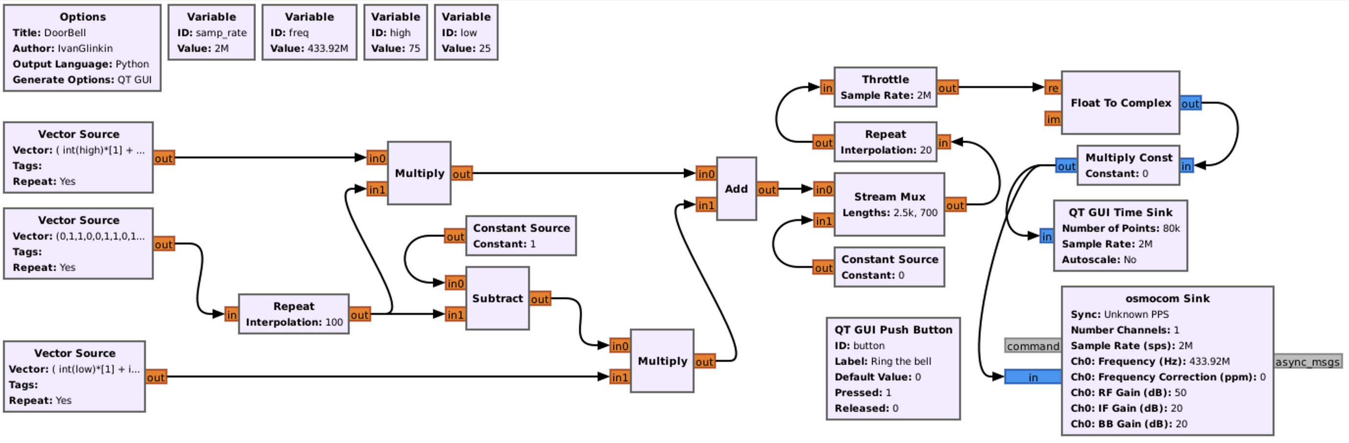
Overall, the final flowgraph should be like that. That may look a little bit complicated, but don’t worry, we will explain each block.
Variables are pretty straightforward. Sample rate and Frequency are our old friends, right? 2 MHz for the Sample rate and 433.92 MHz for the Frequency.
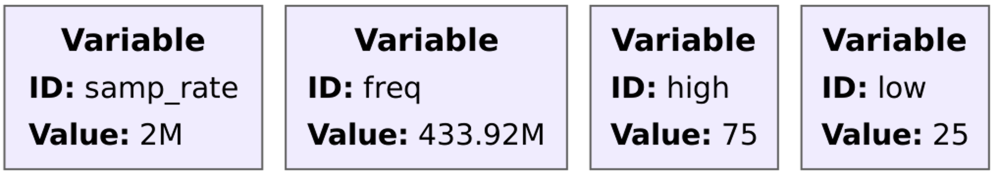
But what are there “high” and “low” with 75 and 25 values?
Remember when we analyzed the signal, we divided each item for 4 pieces? So, 1 is 1110 and 0 is 1000. Which means that in 1 item there is only 75% of peaks, and in 0 item – 25%. Hence those variables are made to calculate each item’s time with peaks.
Next, is the vector source (the middle one in our chart) like we had in the previous paragraph. Nothing specific, but instead of putting 128 numbers, we can only put 25 as it is in our payload.
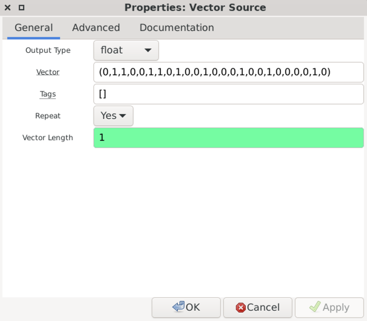
Next 2 sections will be the magic 😉 Let’s start from generating items 1.
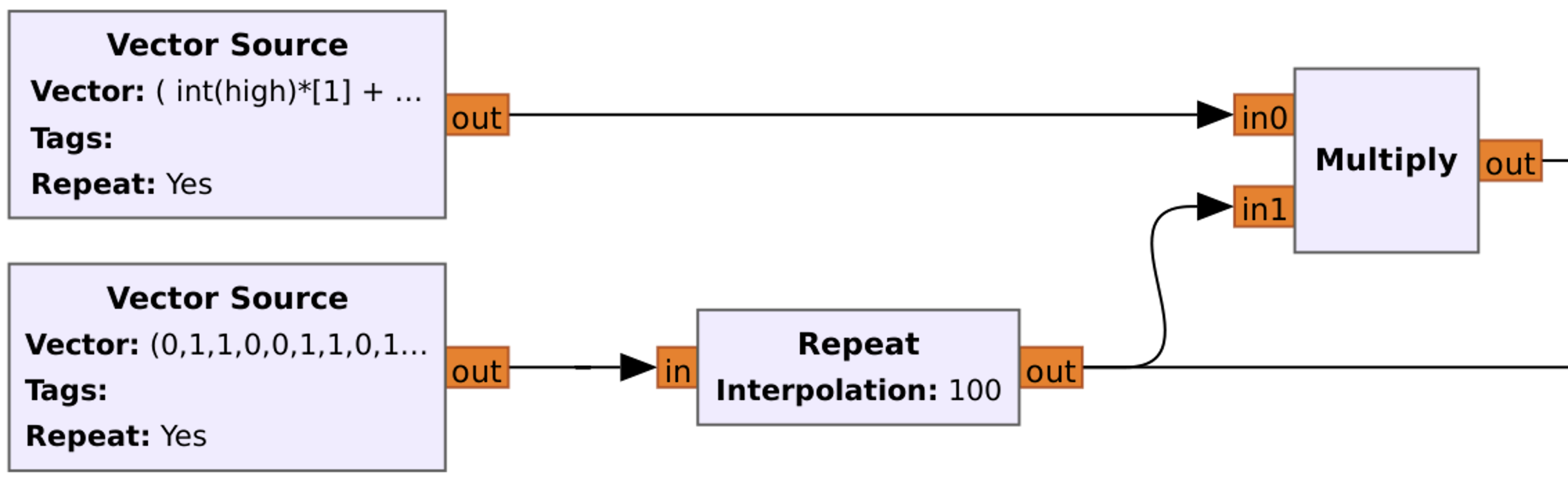
So, what do we have here? The bottom vector source we’ve just discovered. Then, each item is repeating 100 times (Repeat block with Interpolation of 100). So, instead of sending 0, we are sending 00000…00000 (100x times). Next, as you may guess, 11111…11111 (100x time), once again 11111…11111 (100x times) and so on.
After that our signal and basically each item out of 2500 (25 based items take 100 times) is multiplying. But with what? Let’s consider that closely.
The upper vector source variable is the next:
( int(high)*[1] + int(low)*[0] )
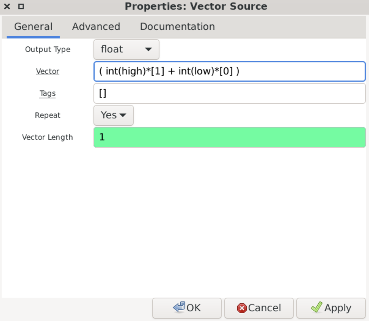
So, we are taking 75 (high variable) times 1 item plus 25 (low variable) times 0 item. Basically, we are generating the next signal:
1111111111111111111111111111111111111111111111111111111111111111111111111110000000000000000000000000
That is too long number for the article hence let’s divide everything by 5:
11111111111111100000
Now let’s multiply (last block) the payload vector (bottom one) with the peak vector (upper).
For item 1:
Payload | 1 | 1 | 1 | 1 | 1 | 1 | 1 | 1 | 1 | 1 | 1 | 1 | 1 | 1 | 1 | 1 | 1 | 1 | 1 | 1 |
1×75% | 1 | 1 | 1 | 1 | 1 | 1 | 1 | 1 | 1 | 1 | 1 | 1 | 1 | 1 | 1 | 0 | 0 | 0 | 0 | 0 |
Multiply | 1 | 1 | 1 | 1 | 1 | 1 | 1 | 1 | 1 | 1 | 1 | 1 | 1 | 1 | 1 | 0 | 0 | 0 | 0 | 0 |
For item 0:
Payload | 0 | 0 | 0 | 0 | 0 | 0 | 0 | 0 | 0 | 0 | 0 | 0 | 0 | 0 | 0 | 0 | 0 | 0 | 0 | 0 |
1×75% | 1 | 1 | 1 | 1 | 1 | 1 | 1 | 1 | 1 | 1 | 1 | 1 | 1 | 1 | 1 | 0 | 0 | 0 | 0 | 0 |
Multiply | 0 | 0 | 0 | 0 | 0 | 0 | 0 | 0 | 0 | 0 | 0 | 0 | 0 | 0 | 0 | 0 | 0 | 0 | 0 | 0 |
So, in our case, with the first 011… items, the signal after the last multiplying box is the next:
000000000000000000001111111111111110000011111111111111100000…
Ok, great. Now let’s consider the bottom part of the graph.
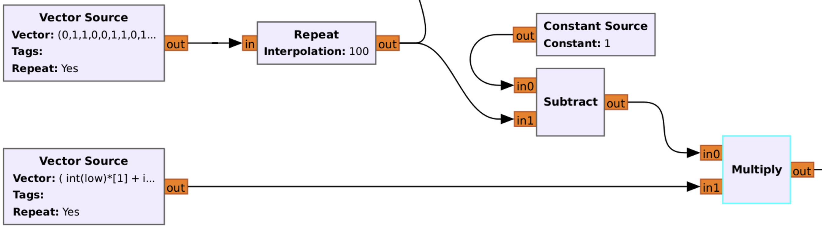
Basically, the first part is the same – main Vector Source, each item repeats 100 times.
Before going to Subtract block, let’s see at the bottom Vector Source:
( int(low)*[1] + int(high)*[0] )
So, we are taking 25 (low variable) times 1 item plus 75 (high variable) times 0 item. Basically, we are generating the next signal:
1111111111111111111111111000000000000000000000000000000000000000000000000000000000000000000000000000
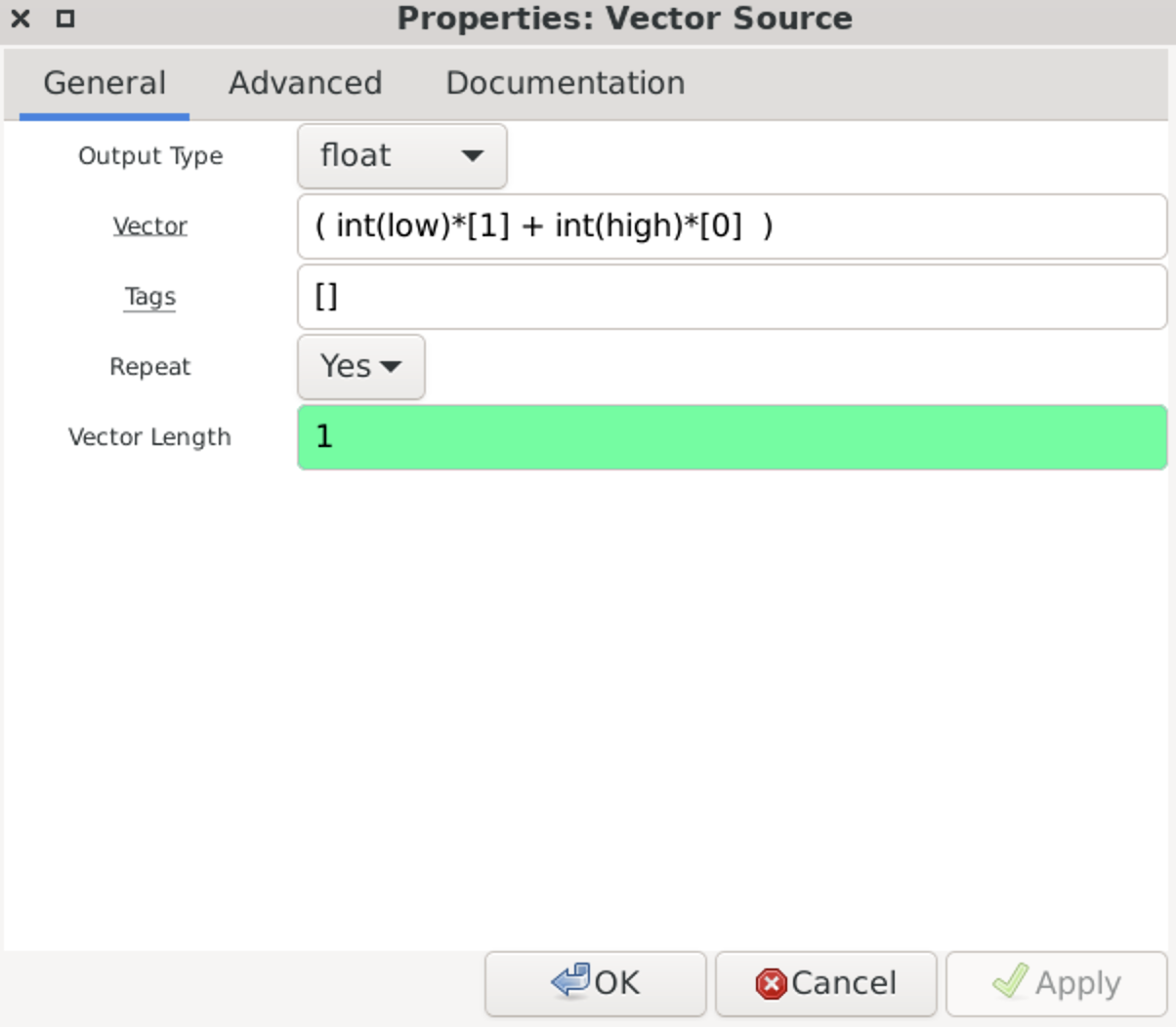
That is too long number for the article hence let’s divide everything by 5:
11111000000000000000
Yeah, almost the same, but with a different proportion (25 instead of 75).
Next step is mind-blowing 🙂 Subtract block, which will subtract data across all input streams.
As the first input parameters we have “Constant Source” which is always 1 and the second one is our main vector payload.
Let’s calculate (all figures divided by 100):
Constant Source | 1 | 1 | 1 | 1 | 1 | 1 | 1 | 1 | 1 | 1 | 1 | 1 | 1 | 1 | 1 | 1 | 1 | 1 | 1 | 1 | 1 | 1 | 1 | 1 | 1 |
Payload | 0 | 1 | 1 | 0 | 0 | 1 | 1 | 0 | 1 | 0 | 0 | 1 | 0 | 0 | 0 | 1 | 0 | 0 | 1 | 0 | 0 | 0 | 0 | 1 | 0 |
Subtract | 1 | 0 | 0 | 1 | 1 | 0 | 0 | 1 | 0 | 1 | 1 | 0 | 1 | 1 | 1 | 0 | 1 | 1 | 0 | 1 | 1 | 1 | 1 | 0 | 1 |
Like from other example, let’s take first 3 result items – 100.
Then, we have to multiply Subtract with our Vector source
For item 1 (0 in original signal):
Payload | 1 | 1 | 1 | 1 | 1 | 1 | 1 | 1 | 1 | 1 | 1 | 1 | 1 | 1 | 1 | 1 | 1 | 1 | 1 | 1 |
1×25% | 1 | 1 | 1 | 1 | 1 | 0 | 0 | 0 | 0 | 0 | 0 | 0 | 0 | 0 | 0 | 0 | 0 | 0 | 0 | 0 |
Multiply | 1 | 1 | 1 | 1 | 1 | 0 | 0 | 0 | 0 | 0 | 0 | 0 | 0 | 0 | 0 | 0 | 0 | 0 | 0 | 0 |
For item 0 (1 in original signal):
Payload | 0 | 0 | 0 | 0 | 0 | 0 | 0 | 0 | 0 | 0 | 0 | 0 | 0 | 0 | 0 | 0 | 0 | 0 | 0 | 0 |
1×25% | 1 | 1 | 1 | 1 | 1 | 0 | 0 | 0 | 0 | 0 | 0 | 0 | 0 | 0 | 0 | 0 | 0 | 0 | 0 | 0 |
Multiply | 0 | 0 | 0 | 0 | 0 | 0 | 0 | 0 | 0 | 0 | 0 | 0 | 0 | 0 | 0 | 0 | 0 | 0 | 0 | 0 |
So, in our case, with the first 100… (originally 011…) items, the signal after the last multiplying box is the next:
111110000000000000000000000000000000000000000000000000000000…
Next one is Add block which is literally addition (1+0=1, 0+1=1, …).
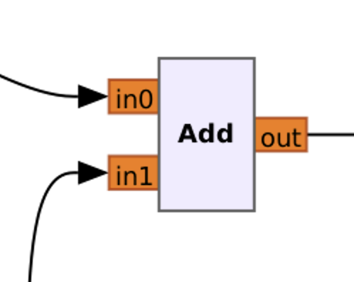
Hence, the graph just adds upper signal to the bottom one:
Upper 000000000000000000001111111111111110000011111111111111100000
Bottom 111110000000000000000000000000000000000000000000000000000000
Add 111110000000000000001111111111111110000011111111111111100000
If divide by 5, hence 100011101110… Seems familiar, right? 😉
As you can see, we get the accurate signal replication. But what’s next?

Next is the Stream Mux block, which multiplex many streams into one with a specified format. Muxes N streams together producing an output stream that contains N0 items from the first stream, N1 items from the second, etc. and repeats.
Referring to our signal – we successfully synthesized the payload, but didn’t do the pause between them. Stream Mux, which is working in series, not in parallel, takes the synthesized signal first, then the pause and repeat.
But do you know why we took 2500 samples as a payload and 700 as a pause? The answer is the payload by itself consists of 25 items, and we repeated it 100 times. And the pause is the length of 7 items hence we have to multiply by 100 as well = 700.
Next is Repeat with a “24” interpolation value and Throttle with the Sample rate of 2 MHz. Let’s first make a deal with a Repeat and then figure out what the Throttle is.
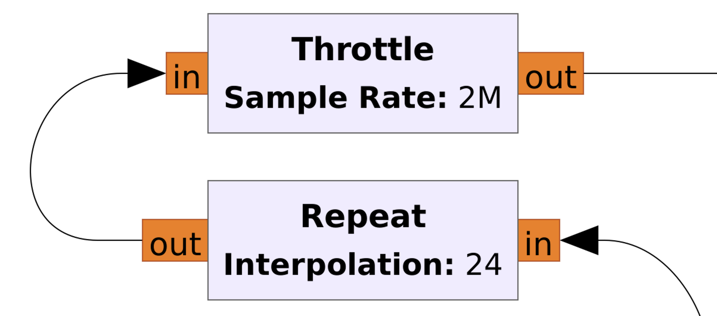
So, we have to repeat each item, including pause, 24 times to make the correct payload. But how we calculated that? There are 2 possible ways:
- As you remember, each item from the first example is 608 samples duration. We took 100 items (25 x 4) for the payload and 28 items (7 x 7) for the pause, which are 128 items overall. If we multiply 128 items by 608 samples duration it’s 77824 samples overall.
Right now, before the Repeat block, we took 2500 items for the payload and 700 items for the pause which means 3200 items overall.
Now we just have to divide 77824 by 3200 and get 24,32. But, the Repeat block can take only integer values hence we have to round it
to 24.
- Each payload item consists of 4 small items. Consequently, when we repeat each payload item 100 times, each small item has been taken 25 times. Now we just have to divide 608 samples by 25 and we will get 24,32. But, the Repeat block can take only integer values hence we have to round it to 24.
As you can see, the simple math. But what about the Throttle, what is that?
The “Throttle” block is a fundamental block used to control the rate at which samples are processed in a signal processing flowgraph. It is often used to limit the processing speed to match the capabilities of the hardware or to control the data rate of the output. The Throttle block essentially introduces a delay between processing blocks, ensuring that data flows through the flowgraph at a controlled rate. This is particularly useful when working with real-time systems, hardware interfaces, or when you need to simulate real-world data rates.
Next block is “Float to Complex” which is simple converting guess what? Right, float data into Complex 🙂
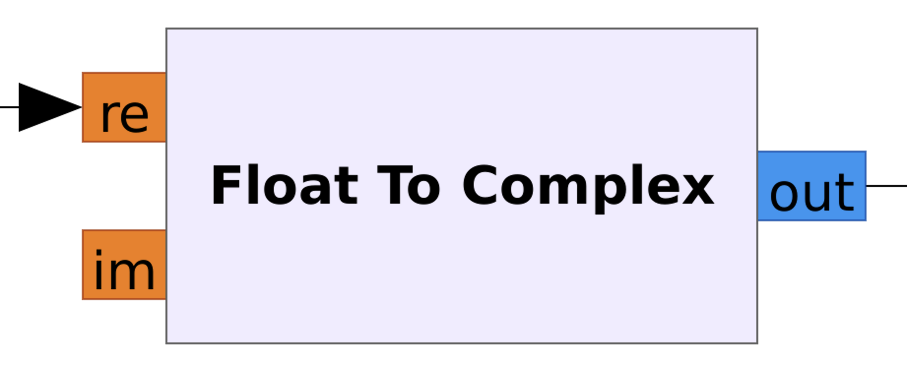
And the final set of blocks is push Button with a Multiply Const, QT GUI Time Sink and Osmocom Sink. We won’t stop on that due to we’ve already discussed several times about those blocks and how they work.

We purchased it from nearest shop for around 12-13 USD, but you can simply google it and order online.
We chose that car on purpose due to the fact that it works on 27MHZ frequency comparing to 95% of the remote-control toys market which is using 2.4 GHz.
So, let’s take a closer look at it.
Disclaimer:
This paragraph will be brief because there’s absolutely no distinction between hacking the doorbell and this specific remote-control car. So, if you’ve read the “7. Hacking a doorbell” section attentively, you can hack this toy in just 3 minutes! 😊
A. Disassemble
The kit consists of 2 main gadgets: the car by itself and the remote control.
Basically, we don’t need to take them apart because even without clues we know how it’s working and what frequency is in use. But let’s at least disassemble the remote control.
So, 4 buttons (unfortunately, not variable resistors), 2 transistors, microchip, capacities and the long antenna. Great, everything is super simple.
Moreover, as you can see, there is a marker highlighted 27M, which, from our understanding, means 27 MHz transmitter.
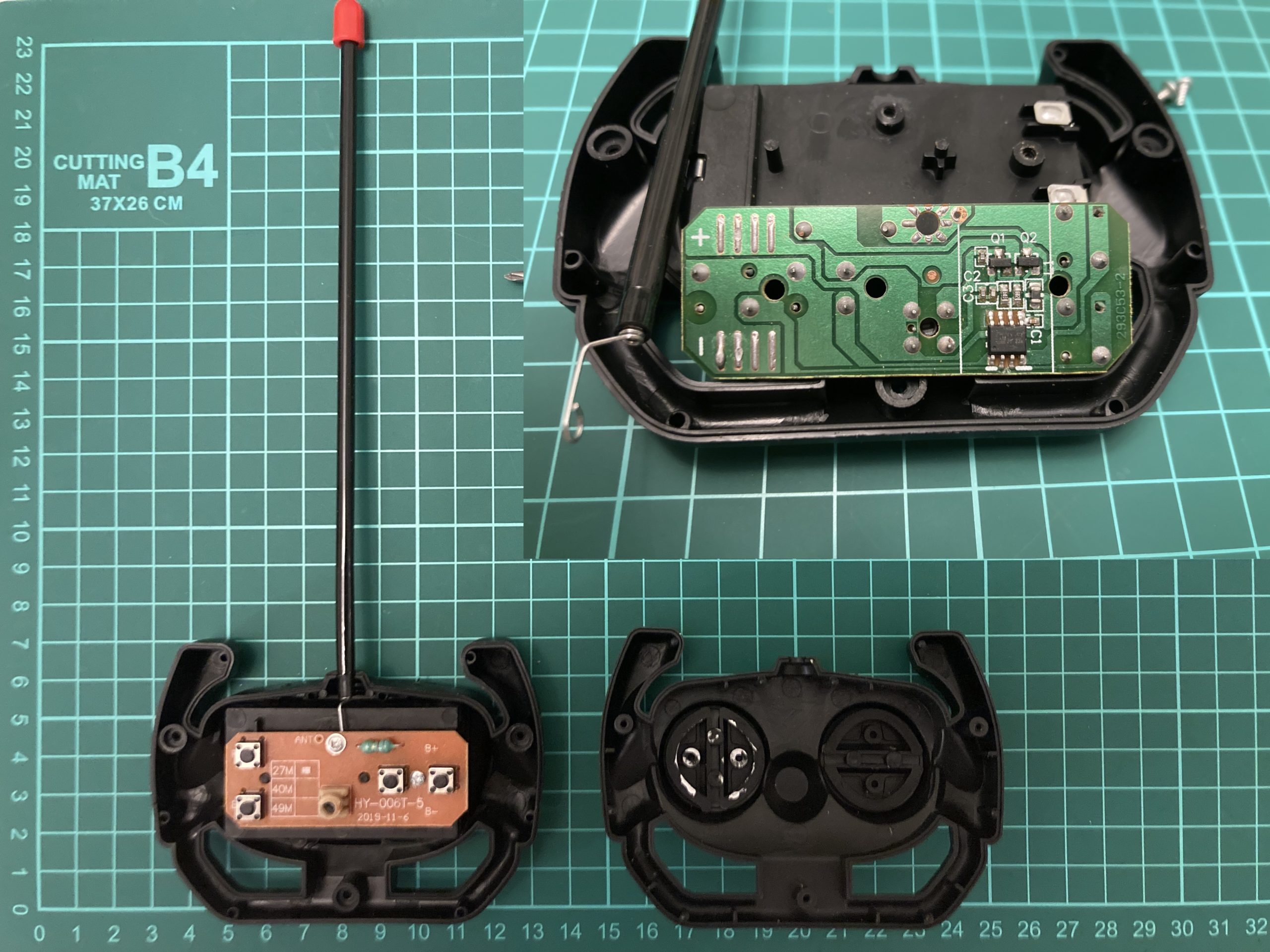
B. Defining the frequency and getting the payload
Like we did with the doorbell, let’s define the working remote-control car frequency. We have already known about 27 MHz, hence let’s open Universal Radio Hacker and set it up.
The settings are:
- Device: select “HackRF”
- Device Identifier: just click the refresh button. But if you have only one connected HackRF no need to do that
- Frequency (Hz): by default, it’s been set as 433,92M. We have to amend that to 27,0 MHz
- Sample rate (Sps): by default, it’s been set as 10,0M. Let’s adjust it as 2,0M
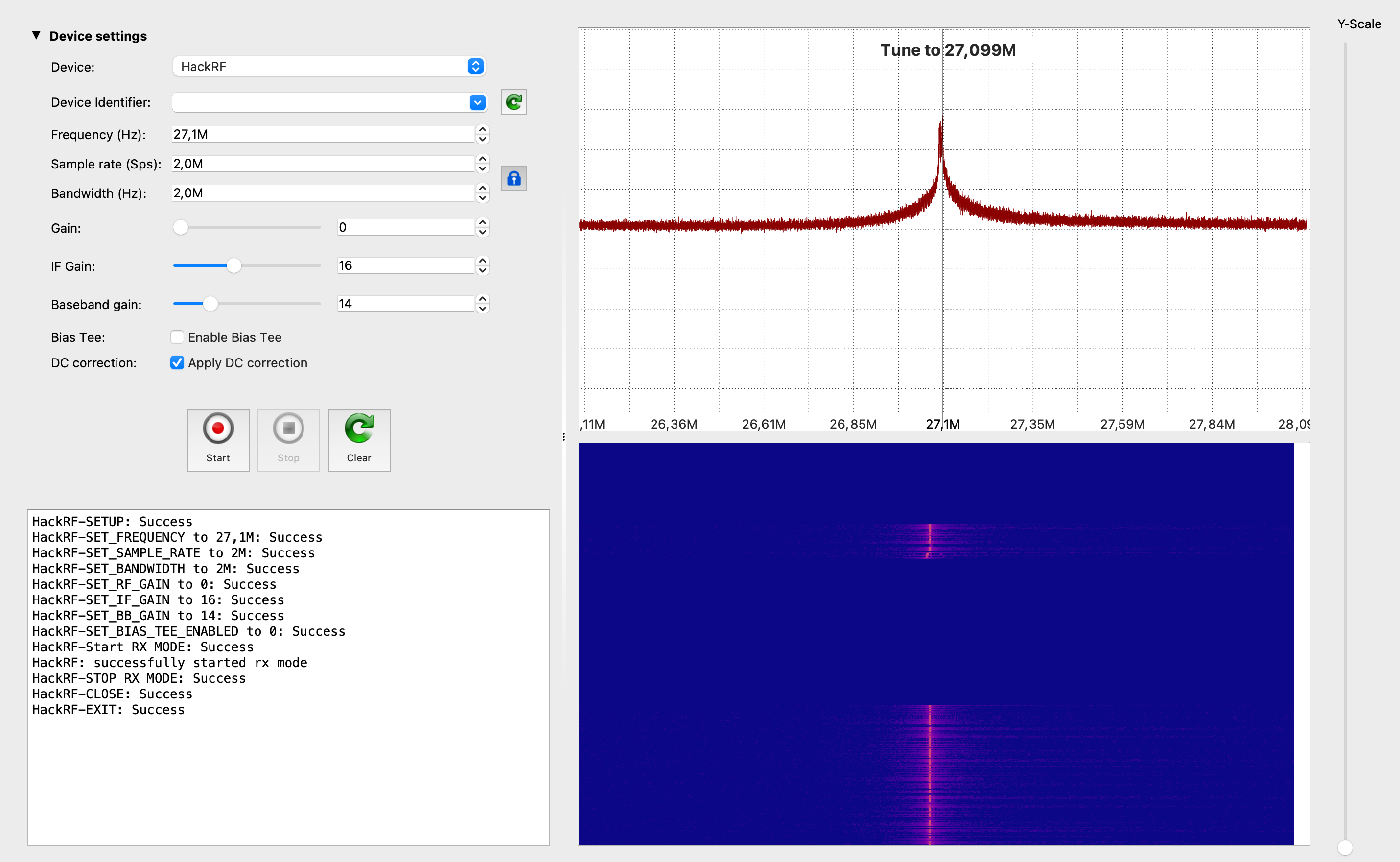
Based on the research, the signal is transmitting on the ~27.1 MHz. Now it’s time to catch the payload.
Following the approach we did with the doorbell, we successfully got the forward drive payload. If we consider the long peak as 1 and double short peaks as 0, the forward drive payload is 111100000 or 111011101110111010101010101010101010 if we divide the payload by short items.
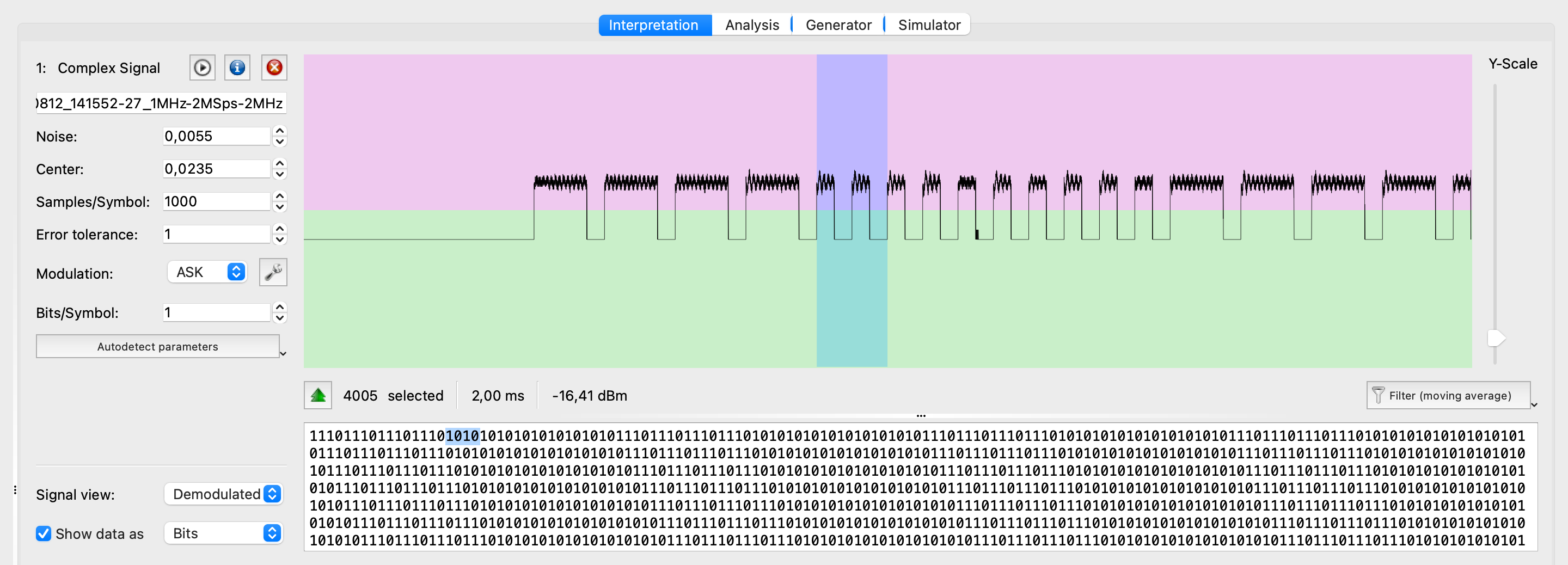
Also, please keep an eye on the duration – ~4000 samples for each of the payload items or ~1000 for the short one. We will need that for the future calculations.
Great, let’s get other payloads: for the reverse drive as well as for the left and right turns.
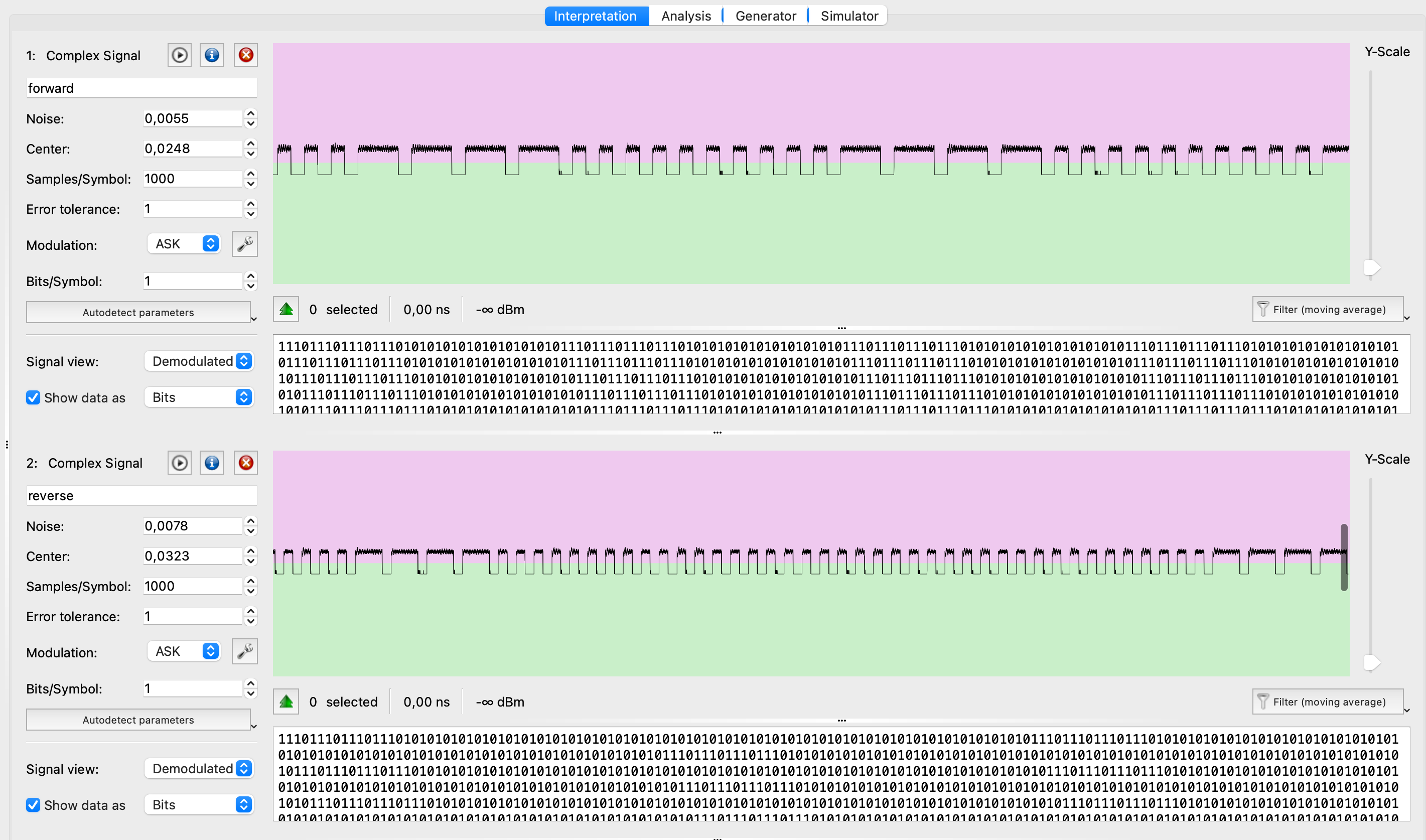
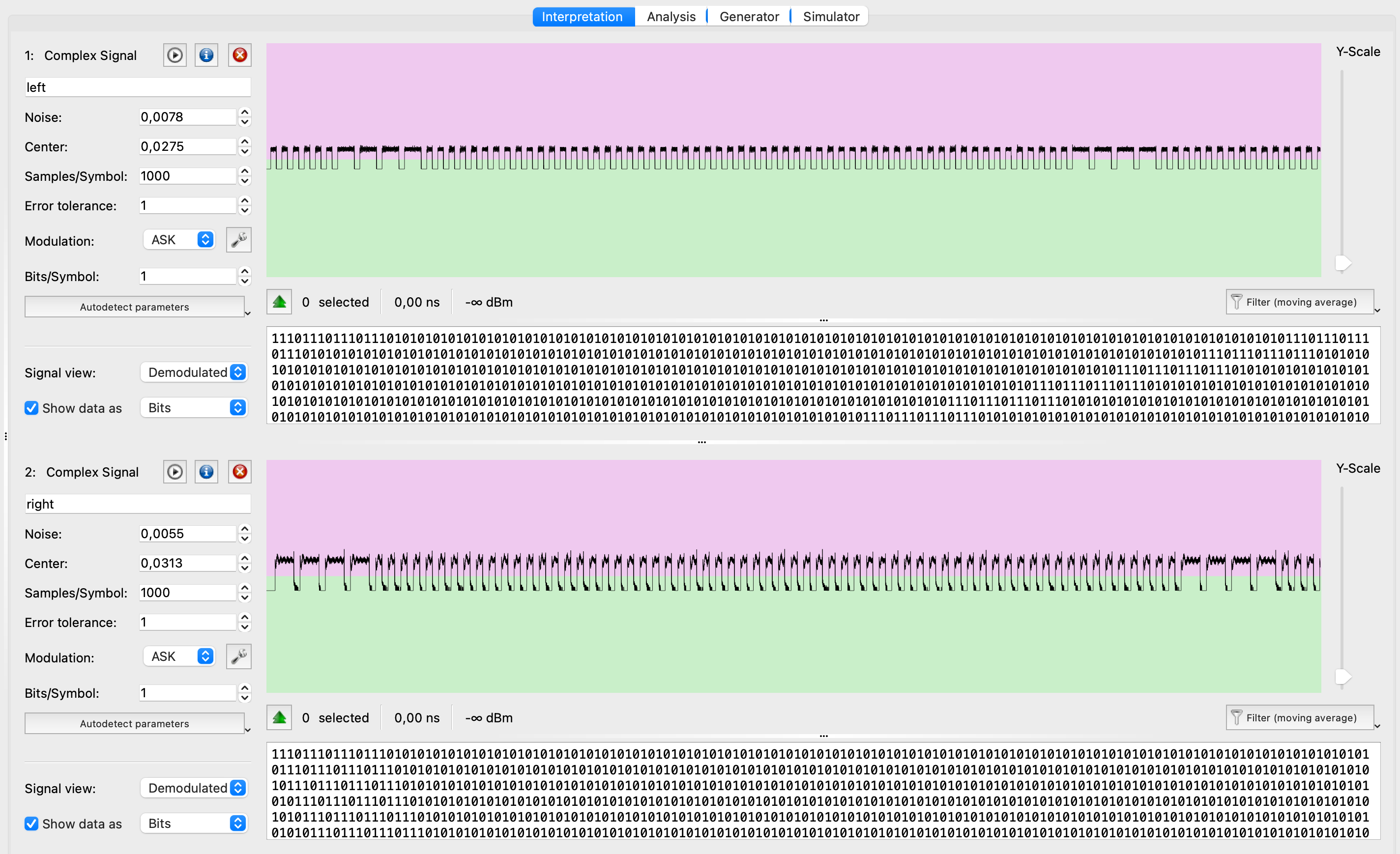
Forward: 111100000 (4×1; 5×0)
Reverse: 111100000000000000000000 (4×1; 20×0)
Left turn: 111100000000000000000000000000000 (4×1; 29×0)
Right turn: 111100000000000000000000000000000000 (4×1; 32×0)
One more Important note. As you can see, there is no pause between signals like we had in the doorbell analysis. In that case, during the synthesizing the signal, we have to send the payload one by one without any delays.
C. Synthesizing
Synthesizing the remote-control car signal as easy as we did it for the doorbell. Indeed, why do we need to create the scheme from the scratch when we can duplicate the existing one with some minor adjustments?
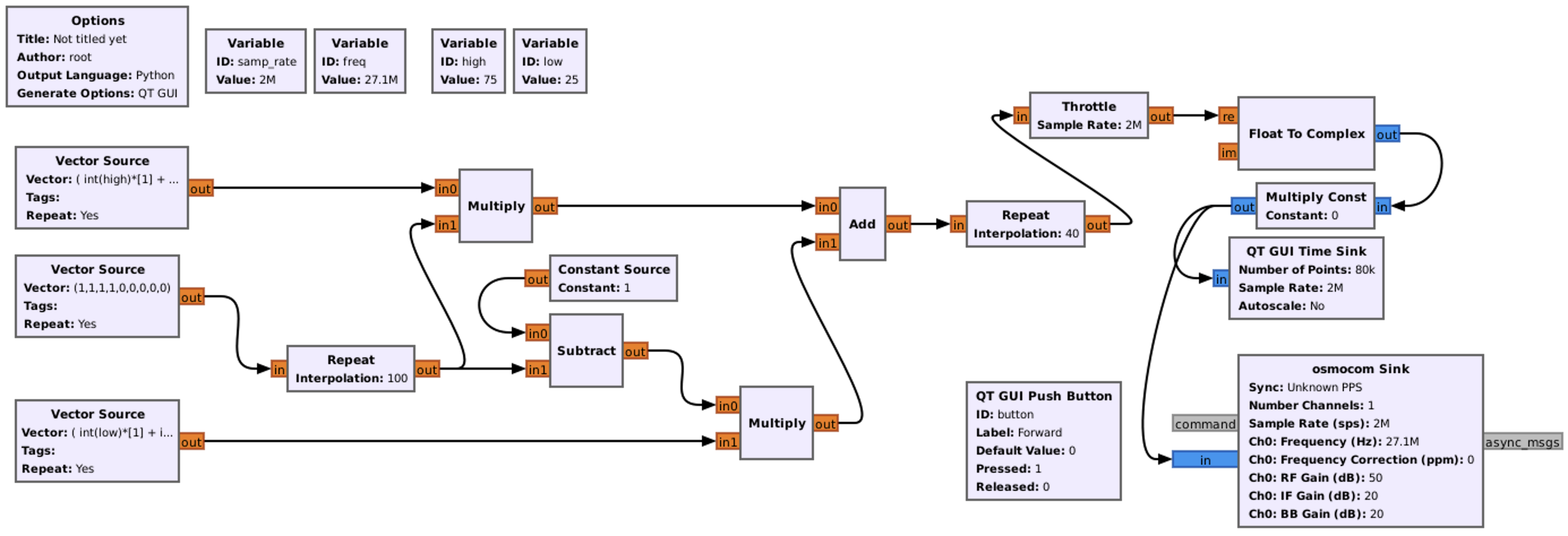
So, the final scheme for the forward driving should be like that. Let’s explain what we’ve changed.
First, and obvious, it’s frequency. The new one is 27100000 Hz. Other variables like sample rate, high and low we kept the same.
Next, the main Vector Source aka the payload. Because we are creating the scheme to make the car drive forward (111100000), the value is (1,1,1,1,0,0,0,0,0).
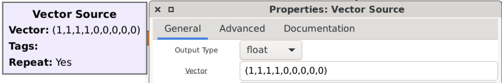
The interesting thing is going with the bottom vector source. Right now to emulate 0 we have to generate 1010 (instead of 1000 previously with the doorbell). In that case we can do it by putting ( int(low)*[1] + int(low)*[0] + int(low)*[1] + int(low)*[0] ).
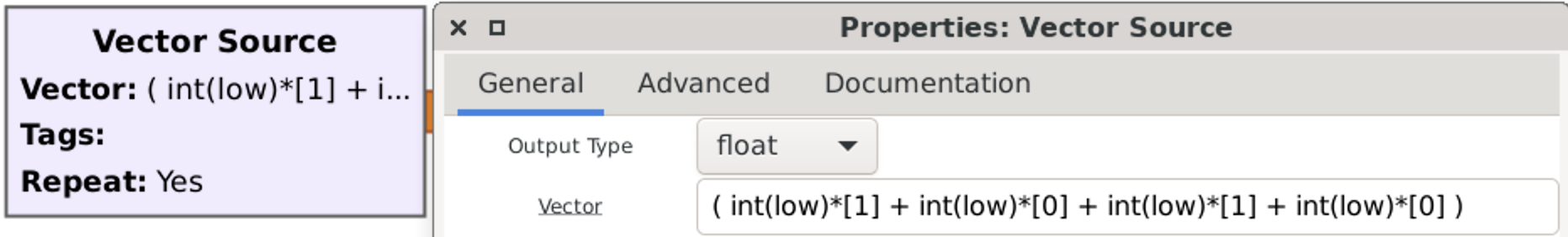
Because we don’t want delays/pause between payloads we can easily remove Stream Mux and dependent Constant Source from our chart.
The last change we have to do to make that working is the last Repeat. Once again, using our formula, 1000 samples duration divided by 25 is 40. Hence, the final answer is 40.
And, of course, don’t forget to change the Button’s caption 🙂
Let’s launch.
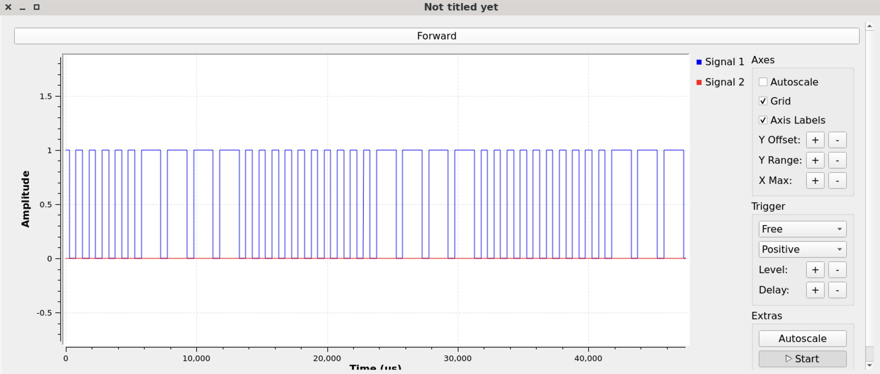
Great, it’s working. Now it’s time to combine all directions into one graph and launch.
But we won’t show it within this article/book and left it as your homework. Also, don’t forget to analyze forward left and right driving as well as reverse left and right driving signals.
As the final result your graph should be something like that.
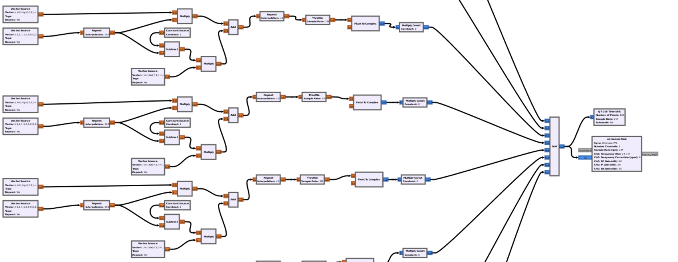

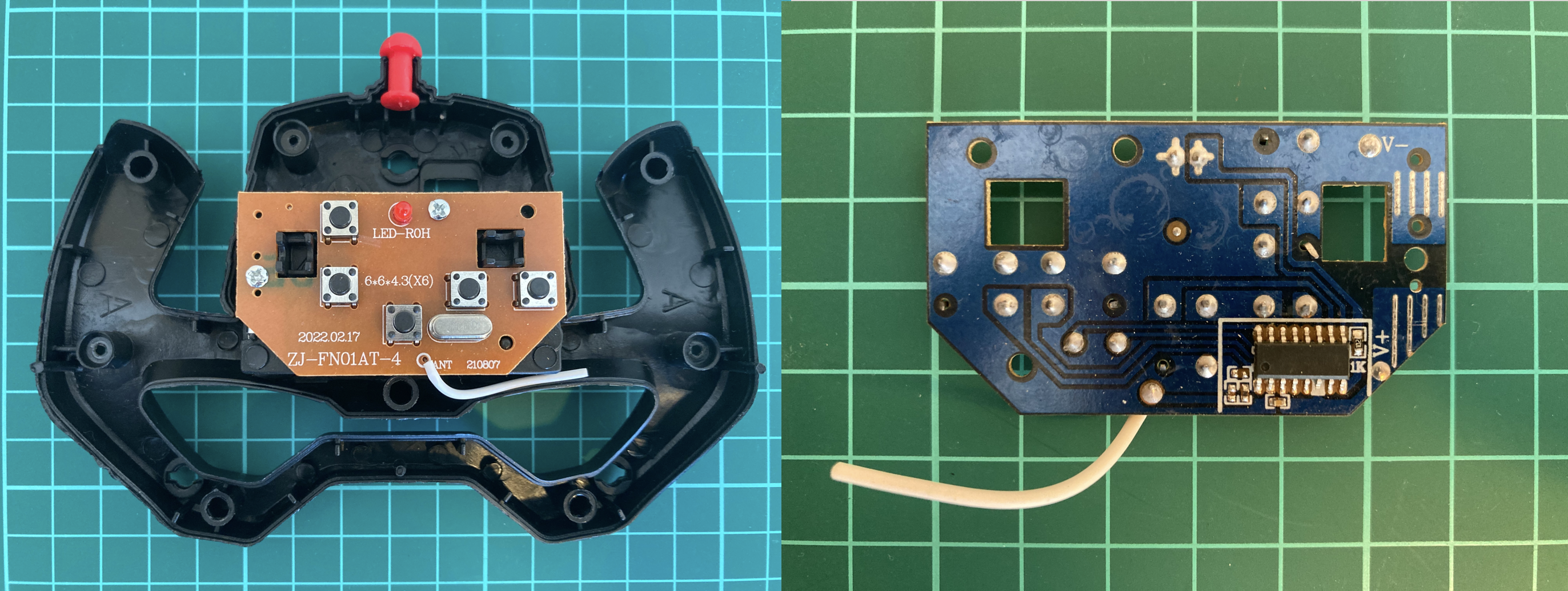
Hm, the scheme is super unified: only 4 buttons with a LED, SAW and microchip. The most embarrassing stuff is the antenna: it’s super short and, once you hold the remote control, limited not only by the plastic body but by your hands as well. In that case the control distance is shorter than it could be. And if look to the description, it’s quite tough not to get laugh – where is the antenna? 🙂
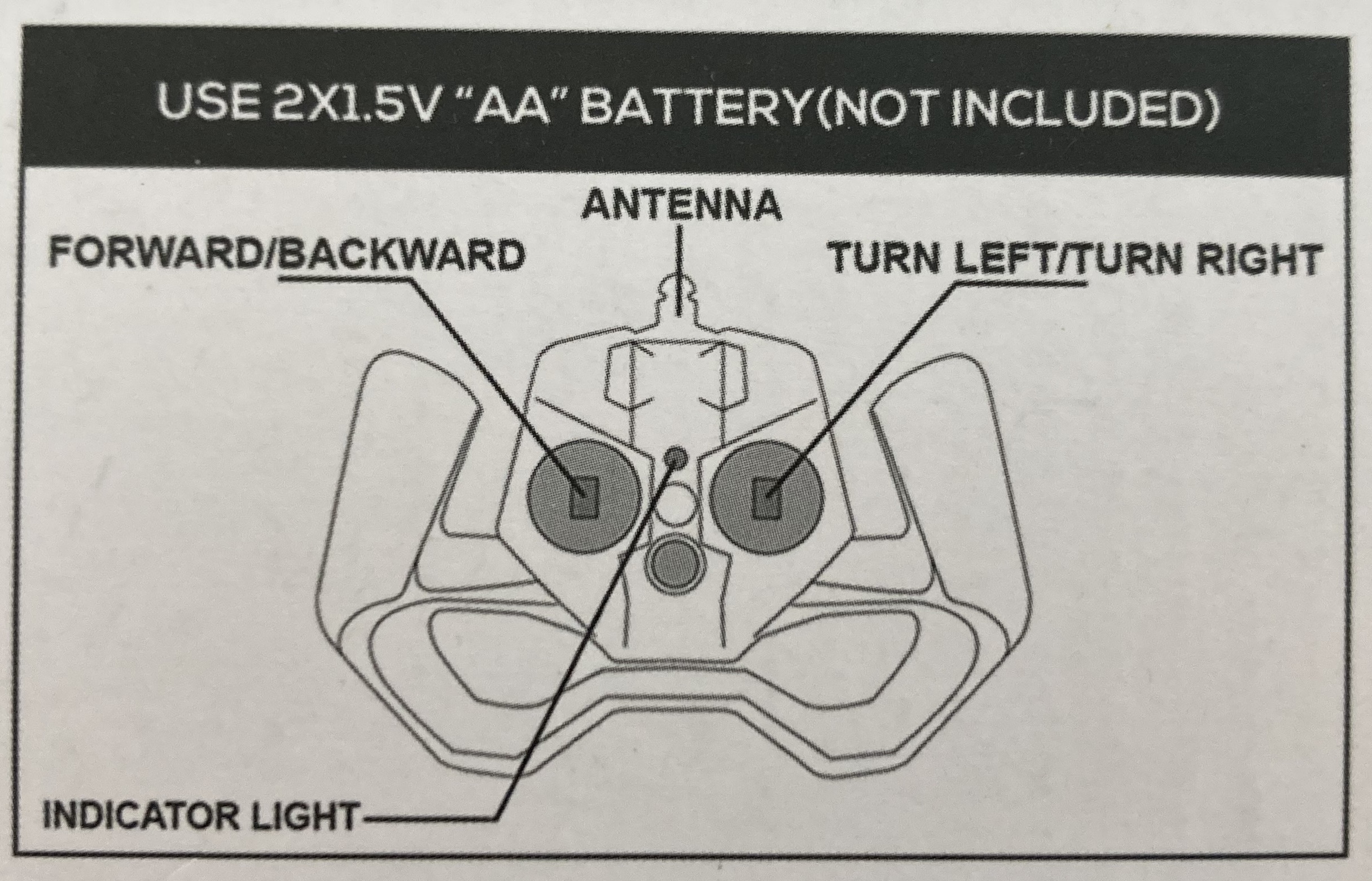
B. 2-way handshake
Like we did with the doorbell and the previous remote-control car, let’s define the working frequency. We have already known about 2.4 GHz, but we can’t define it as easy as we’ve done before.
As you may remember, HackRF has limitations of 20 MHz samples hence using CubicSDR we can cover the range only, for example, from 2400 MHz till 2420 MHz, or from 2430 MHz till 2450 MHz.
In that case, to discover the whole range, we have to use hackrf_sweep feature based on hackrf_spectrum_analyzer.
Let’s get started.
Once we switch on the remote control (when the car is off), we can see that the LED is blinking. But, having switched on the car, the LED on the remote control turns down. That’s quite interesting.
Based on that behavior we can assume that the remote control is trying to establish a connection with the car. When the connection is in place, the car can be controlled and drive any directions.
Let’s launch the hackrf_spectrum_analyzer and analyze signals. Due to the fact that 2.4 GHz frequency is used by Wi-Fi and there are plenty of peaks and noise, we have to adjust setting to reduce those destructions.
First, let’s keep the car off and switch on the remote.
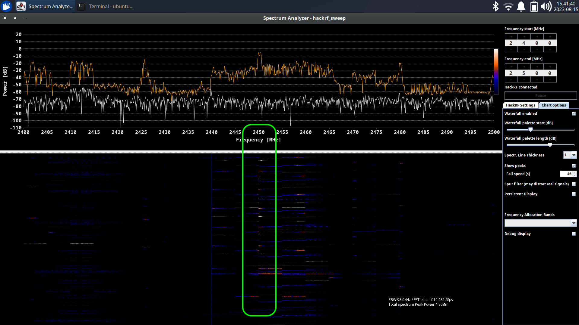
As you can see, immediately after that the signal appears on the ~2450 MHz frequency. Let’s call it “ping”. Great, now we have to switch the car.
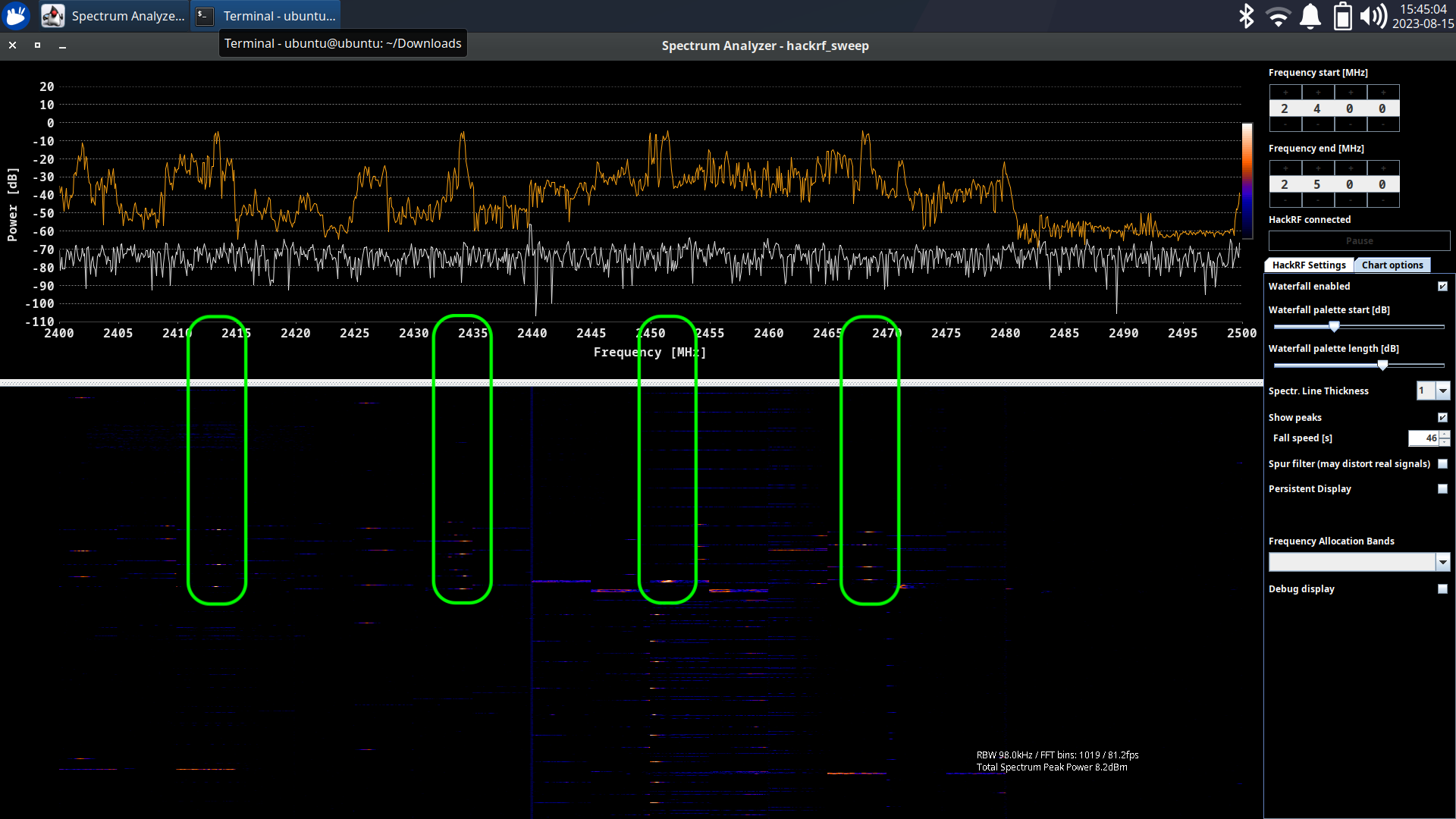
Once we’ve done that, the powerful signal appears next to our “ping” request.
But there are also some phantom peaks on ~2418, ~2434 and ~2468 MHz. We assume it’s just an echo, but let’s keep that in mind.
Interesting fact: after a second the signal interchange stopped. Seems like the connection has been established the car is waiting for the commands. Ok, let’s press the forward driving button.
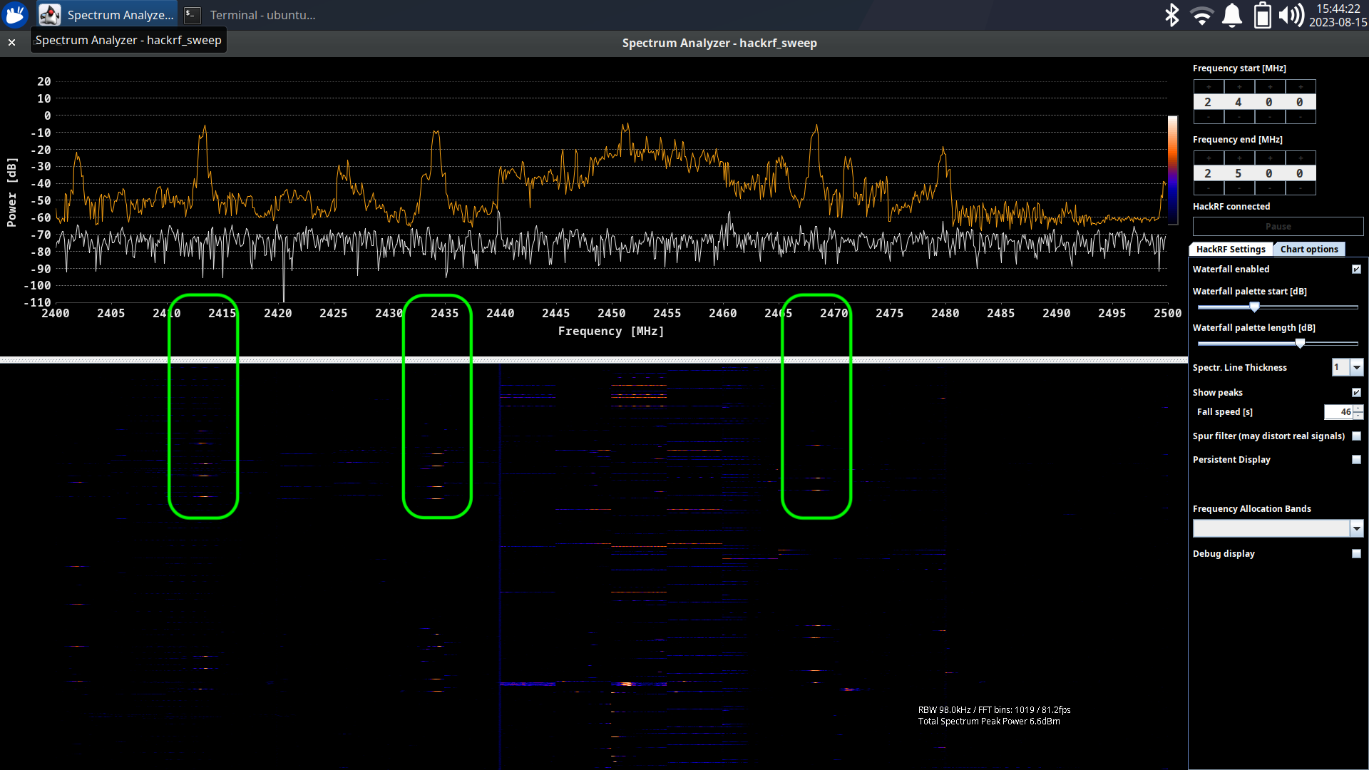
The most powerful signal is on ~2434 MHz frequency. Other two can be an echo, but once again, let’s keep that in mind.
Before going to signal analyzing, let’s wrap up how the communication is working.
First, the remote control starts “pinging” the car by sending the data on the ~2450 MHz frequency.
Once the car receives the data, it replies back to the remote. Remote receives the signal and stops sending pings.
In that case the connection has been established.
Finally, the remote can send payloads and the car can execute them.
C. Payloads catching
Great, we figured out how the remote-control car was working on a high level and found the frequencies ranges. To move forward we have to define the exact numbers so we can catch the payload and reuse that.
Let’s plug in our HackRF, launch the CubicSDR and start with the “ping”, setting the central frequency as 2450 MHz.
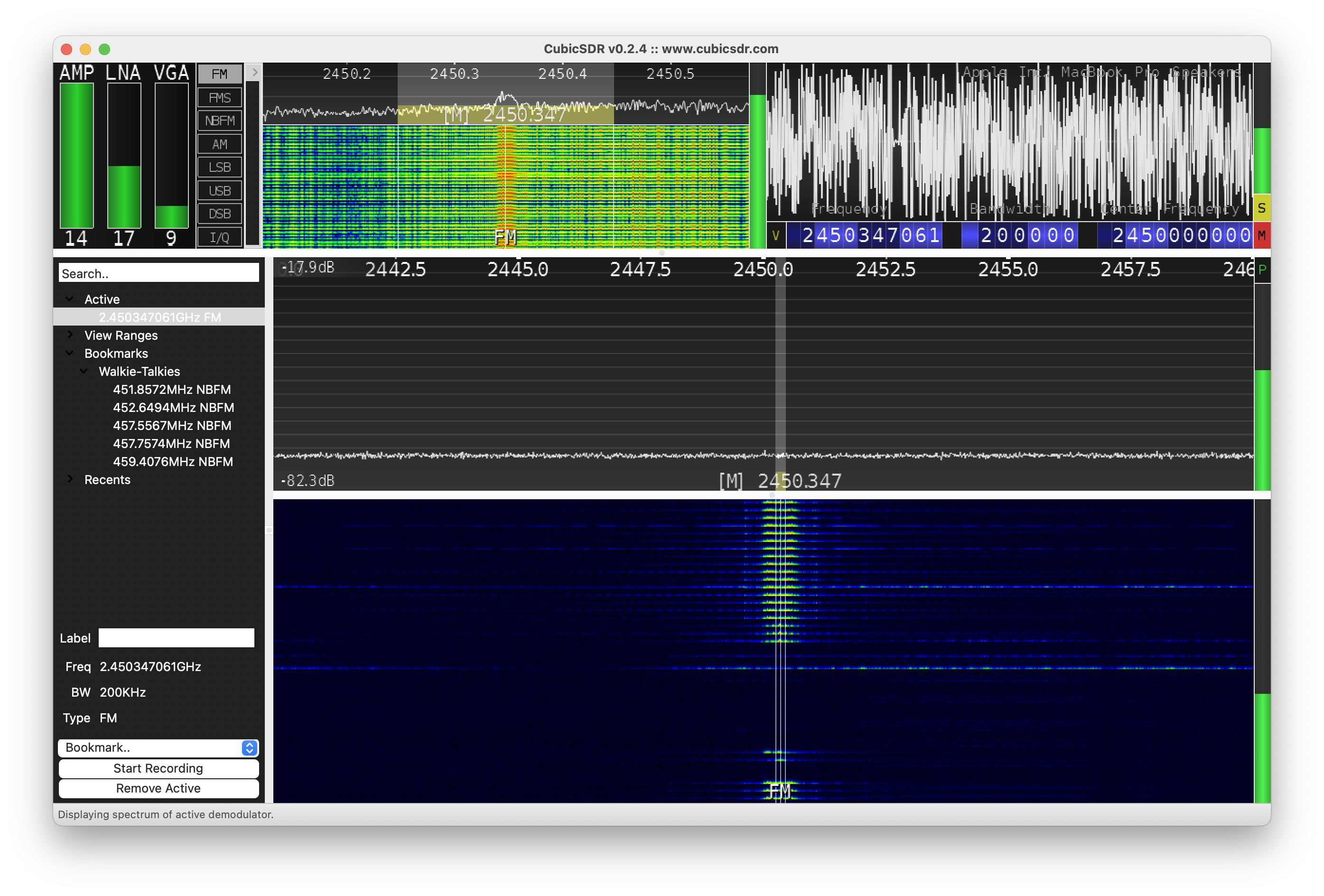
Once we switched on the remote, we started receiving the high peaks on the 2450347061 Hz frequency, which means we found the “ping” signal. For the convenience, let’s use 2450.347 MHz
Next, in case of a 3-way handshake, we would have to get a ping back reply from the car to the remote. But, as we investigated on the previous stage, due to the fact it’s a 2-way handshake: remote requests, the car replies; we actually don’t need to perform that. As a result, we are easily skipping that stage.
Now it’s time to get the controlling payload frequency. Let’s set the central frequency in our CubicSDR to 2434 MHz and press the forward button on the remote.
Immediately the signal appears and we’ve got the right frequency which is 2434345900, but for the convenience we will use 2434.346 MHz.
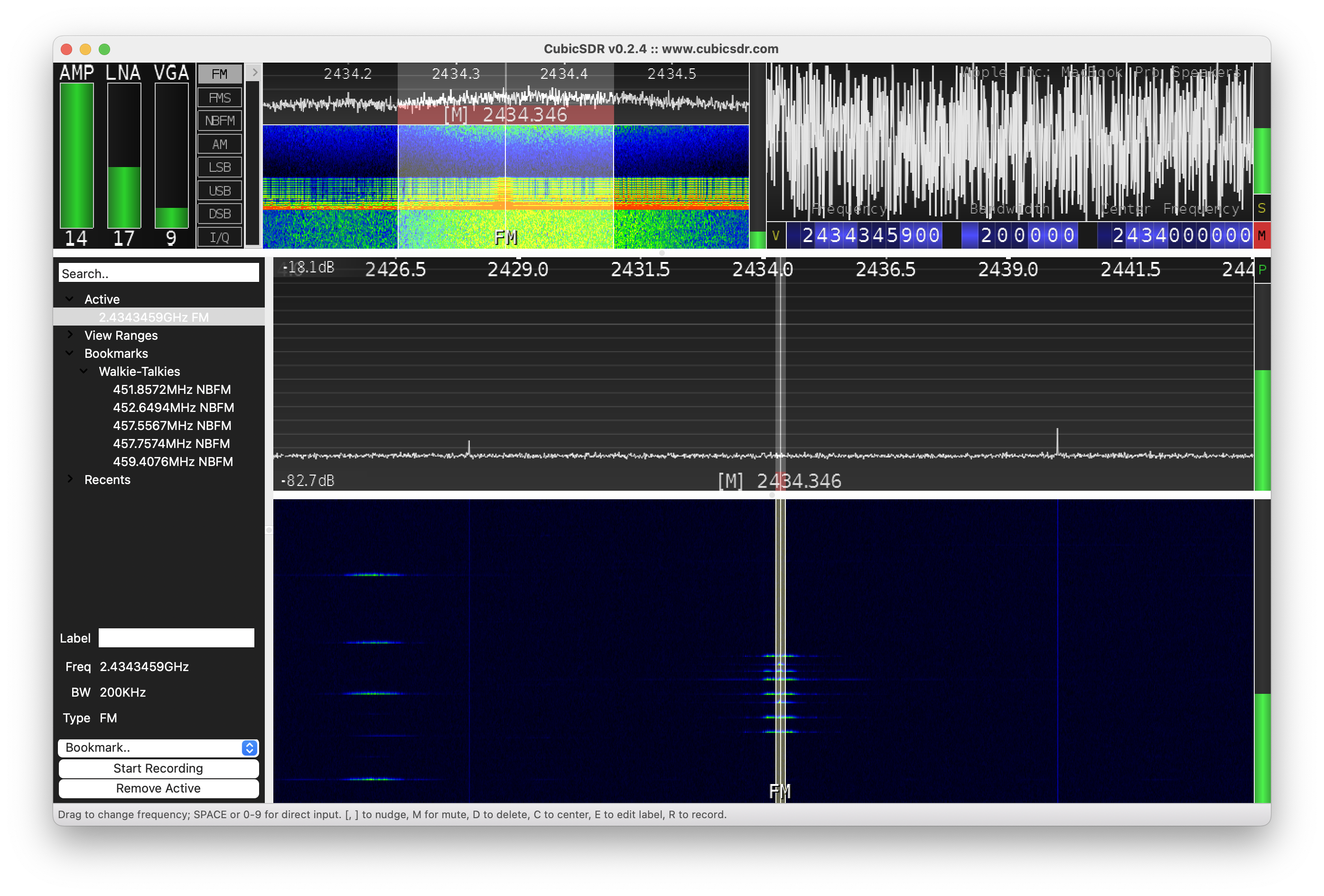
Great, seems like we’ve found working frequencies and it’s time to analyze them.
Let’s open Universal Radio Hacker and set the “ping” frequency which is 2450.347 MHz.
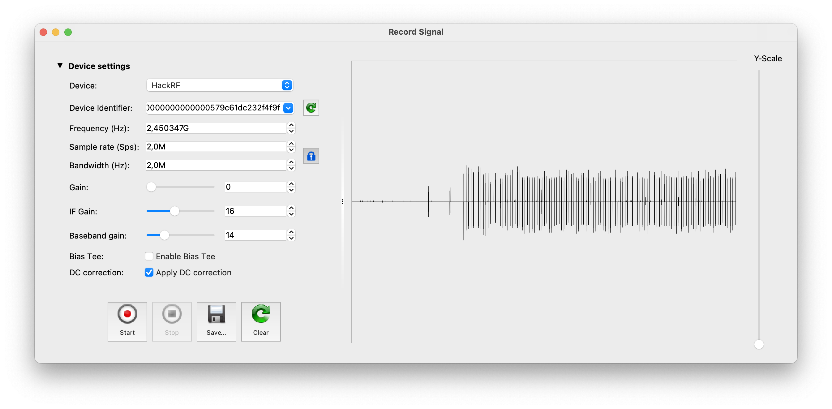
Great, we have the clean signal without the noise. Let’s save it and start analyzing. Hopefully for us the payload is repeatable and does not have the rolling code.
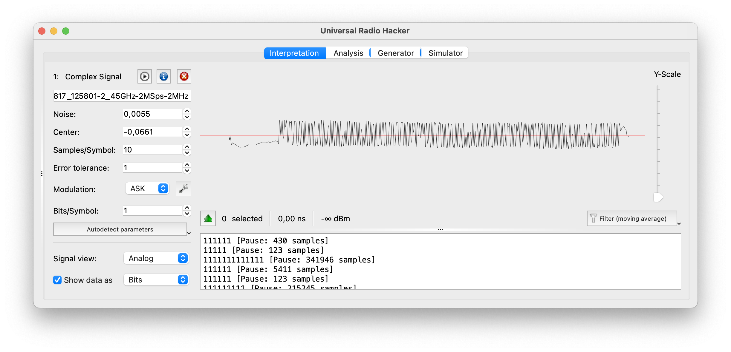
Hm, the payload is quite tough to read. Let’s switch to demodulated view and use the other modulations: ASK, FSK and PSK.
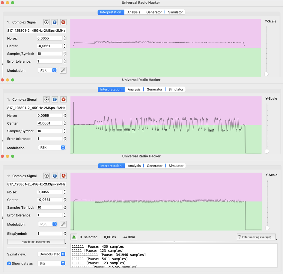
The most useful modulation for us is PSK. But even in that case it will take forever to synthesize the payload.
For the clearance let’s check the moving payloads if they are with the same pattern. As usually, set the proper frequency – 2434345900 Hz and start.
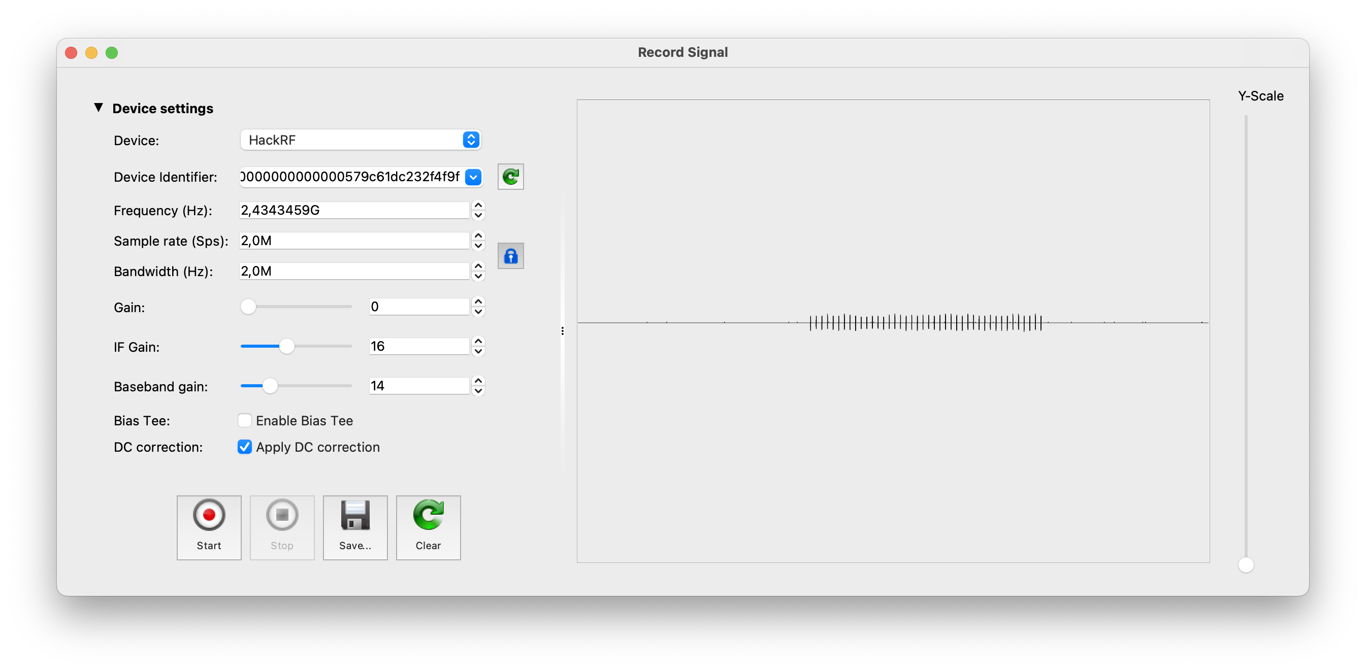
The signal is clear as well, but what is inside?
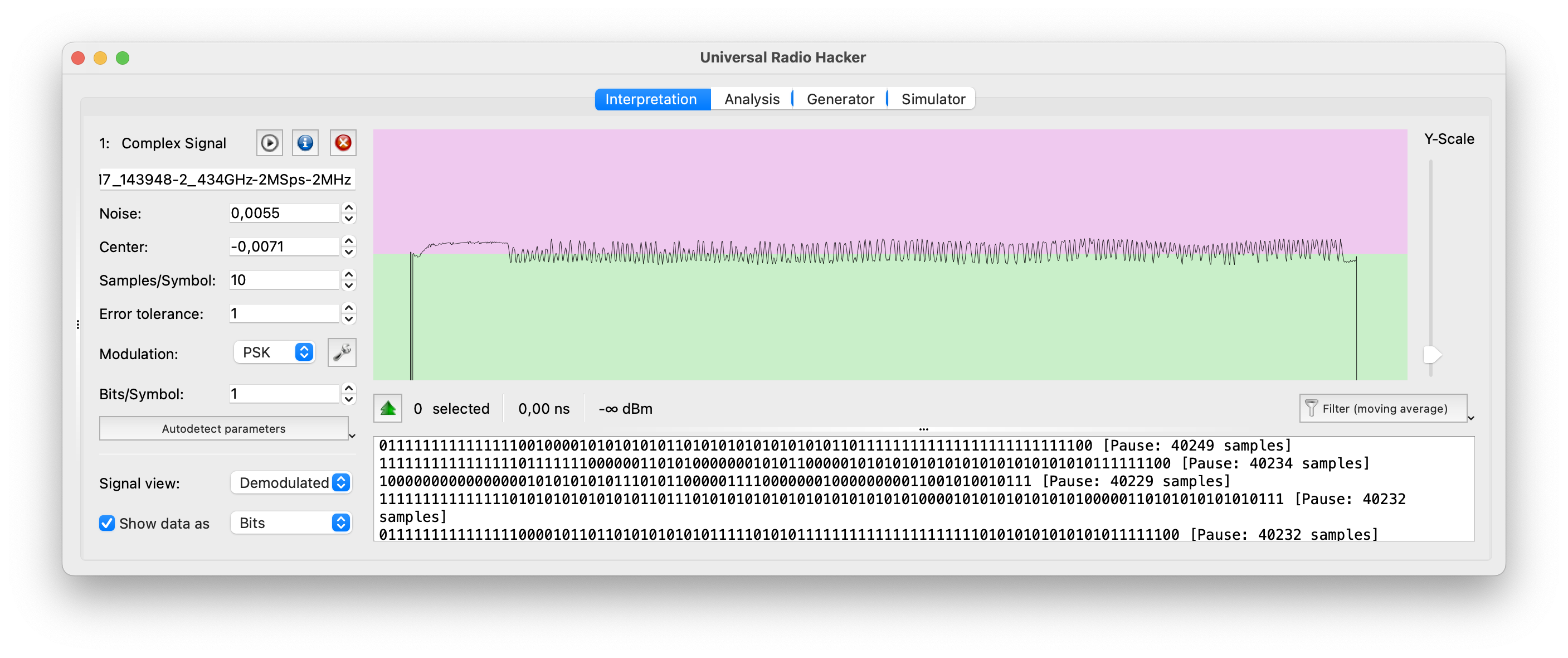
Got it. The pattern is the same and we don’t have that luxury like time to spend for reproducing that. Let’s consider another way.
D. Smart replaying
What if we can create an application which instead of sending synthesized payload will replay the proper saved signal?
So, we will just create the window with 5 buttons: Initiate (the “ping” request), Forward, Reverse, Left and Right. Each button runs the hackrf_transfer application which performs a replay attack. Sounds good hence let’s waste no time and dig into the development.
First, we have to prepare each signal with payload, which will be transferred. To do that, open in URH application the intercepted file from the previous paragraph or intercept it once again.
Then select the best set of signals, put the cursor at the beginning of that set and select everything before that. After that just delete selected.
Next, put the cursor at the end of the pause, select everything after that and remove as well.
As a result you have to have something like that:
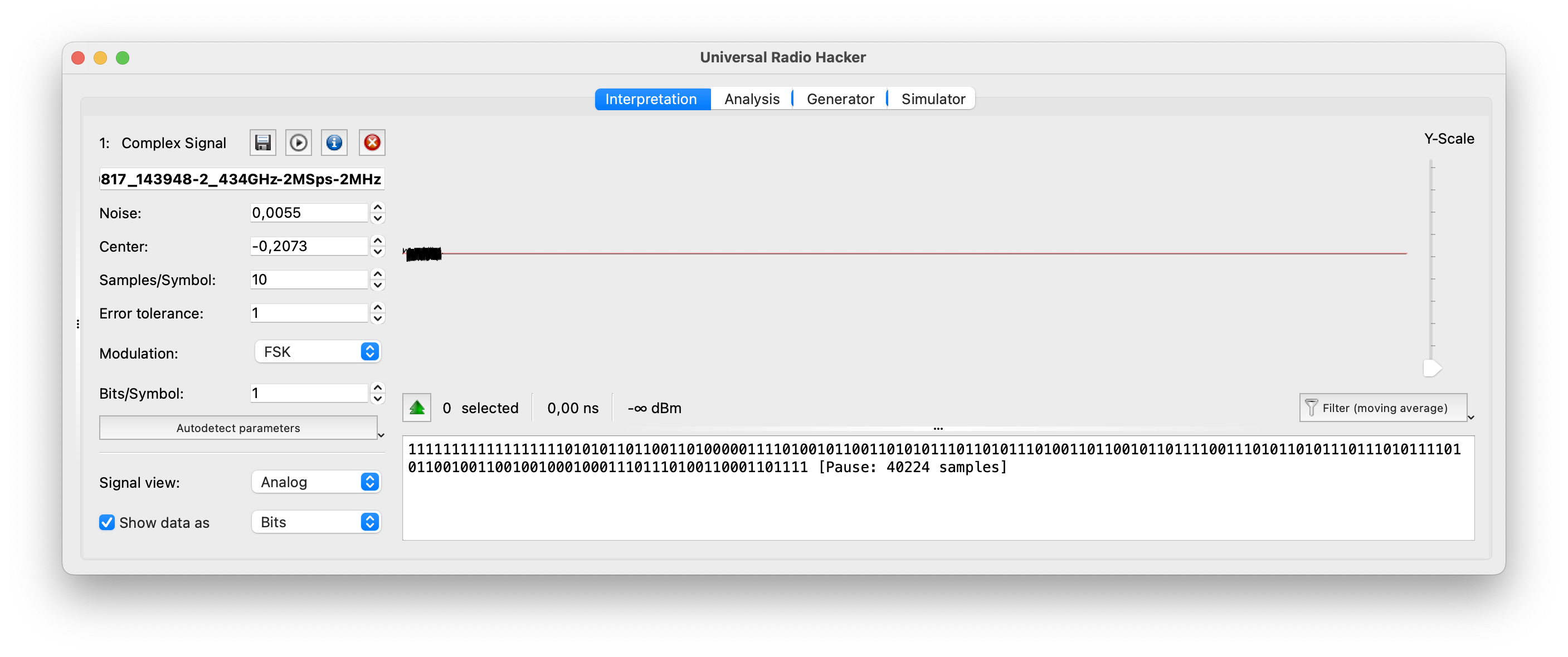
Save the file as “init” and store it in the folder.
Repeat that exercise 4 more times for each moment: forward, reverse, left and right driving.
As a result you have to have 5 files with the proper payloads.
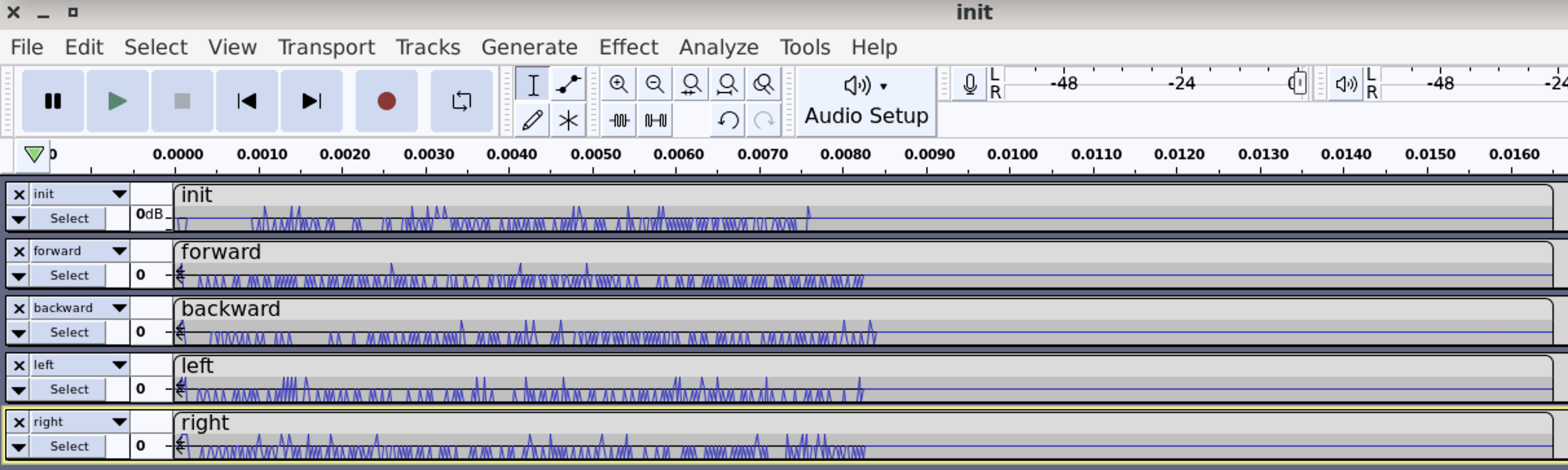
Great, we prepared the payload for each movement. Now it’s time to create the application. Speaking of that let’s use Python3 as our main instrument.
The code is the next:
|
Python programming is not the part of this course hence we won’t explain in details each line. But what we want to show is the part of code, which is in charge of sending a payload.
Please keep an eye on this:
execute_bash_command(“i=0; while [ $i -le 3 ]; do hackrf_transfer -t forward.complex16s -f 2434345200 -s 2000000 -x 45; i=$((i+1)); done”)
Python is requesting Bash, which if executing hackrf_transfer command 3 times in a row. Hence, when we press the button, HackRF starts sending the signal.
Now it’s time to launch that.
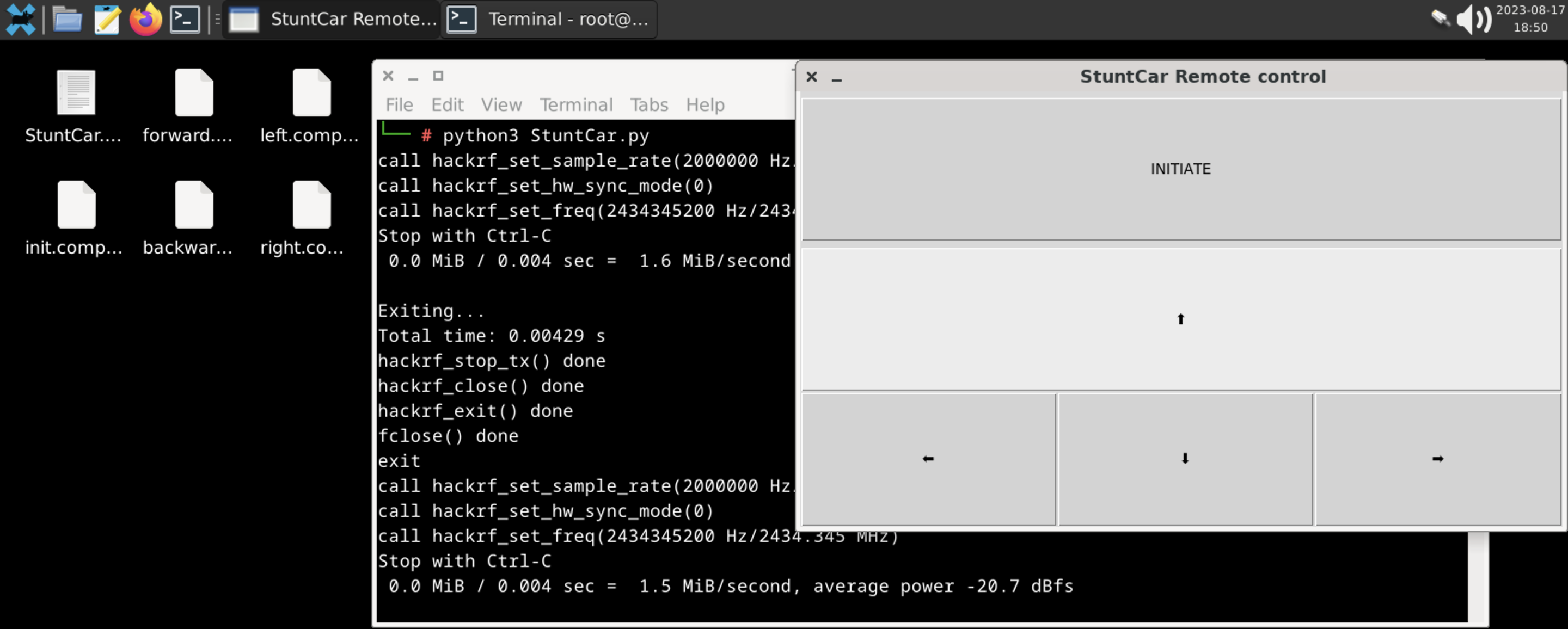
10. Hacking a portable weather station
The final item on our current list to be hacked, but certainly not the least significant, is a portable weather station capable of measuring not only temperature but also humidity.
For our experiments we chose the “Digital Hydrometer” which cost us around 20 USD. And as you may guess it’s wireless and transmitting the data over radio waves. Let’s figure that out.

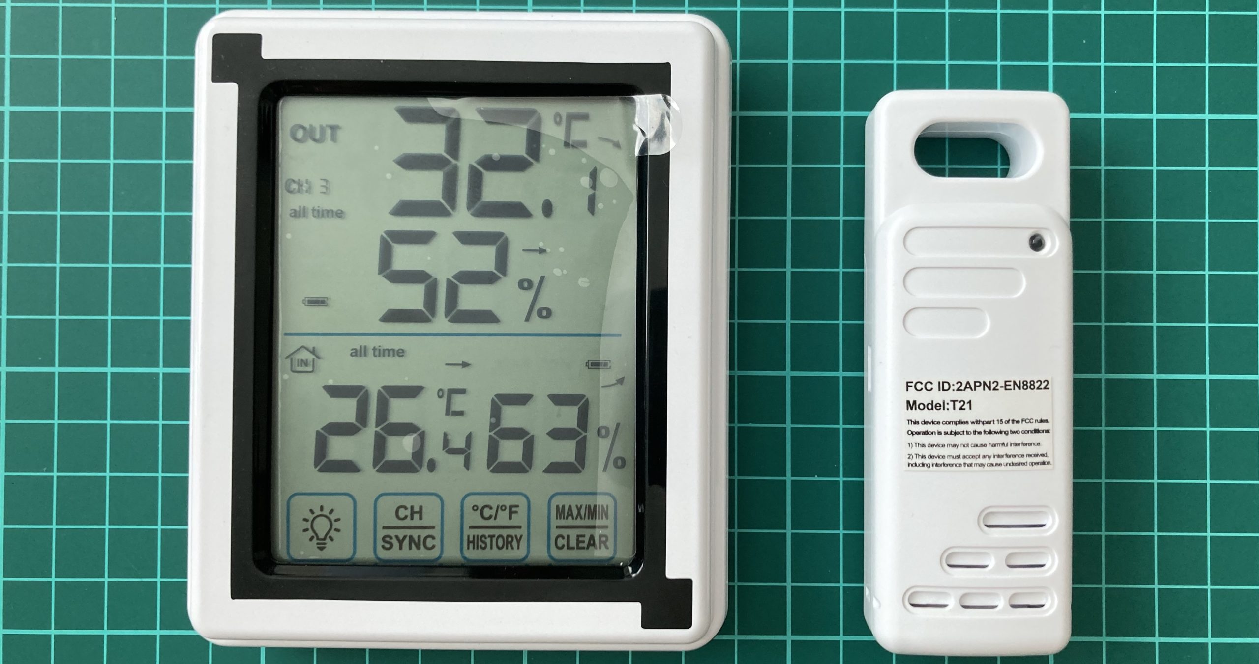
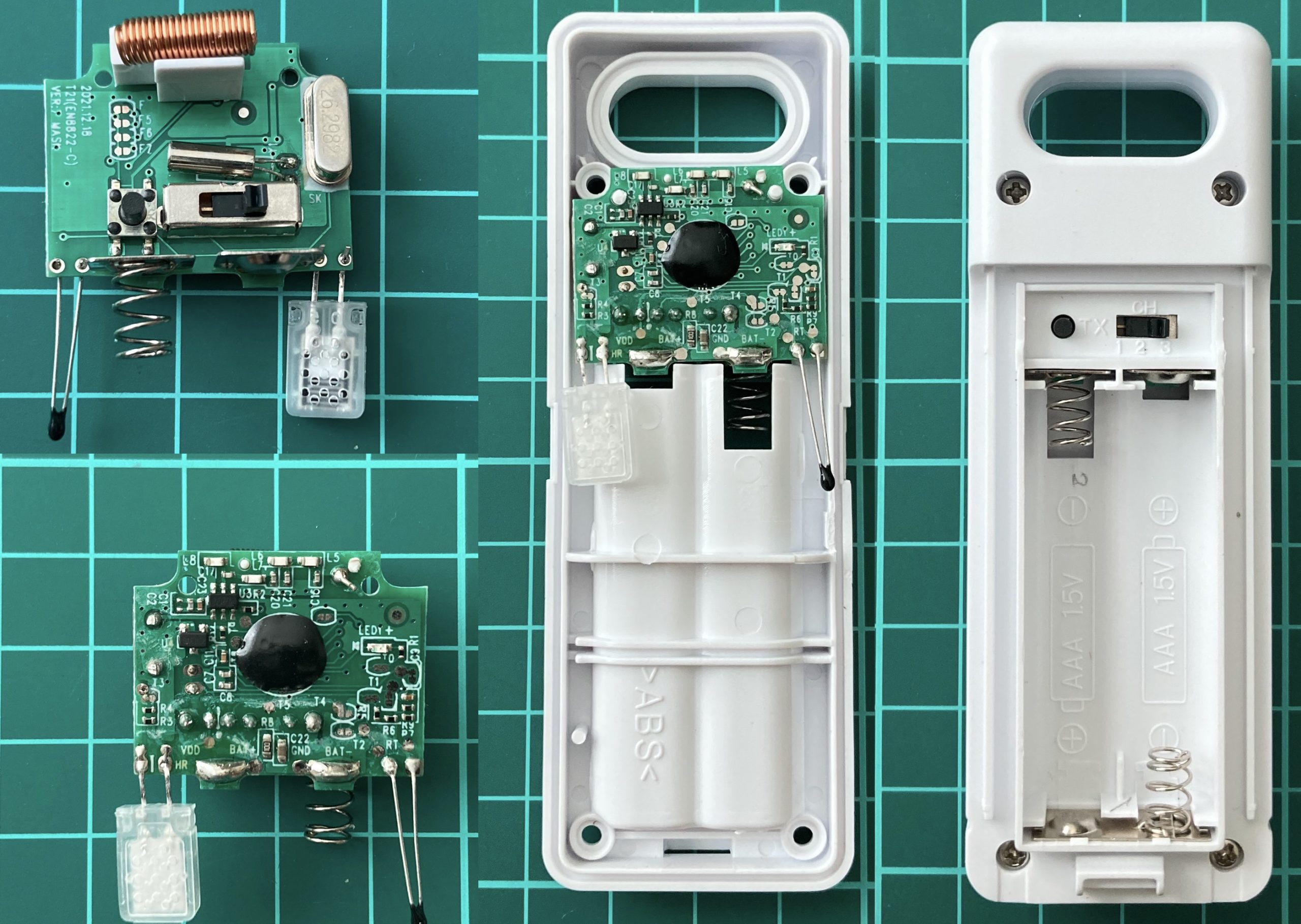
Brief observation tells us about the next.
First, the transmitter, as well as the receiver (weather station), can work on 3 channels (based on the switcher). And we have to check all of them.
Next, there is a button TX for the force transmitting. Thank you for that great feature because during the analyzing stage we don’t have to wait till the signal transmits and can force that.
The antenna is just a twisted cuprum wire like we saw in Flipper Zero. Unfortunately we can’t calculate the length of it but due to the fact it’s working on 433.92 MHz, it should be around 34-35 cm.
There is also a SAW, some transistors, resistors and capacities, and the central microchip as a heart. And, of course, there are 2 sensors for the temperature and humidity measure.
Moreover, as you can see, 2/3 of the whole transmitter is consisted of batteries. If we are talking about outdoor usage or just “purchase and use” it’s a great solution. But please also consider, if you want to get the data from a limited place or use it for your future engineering project, it’s better to take it apart and save the room. 3 volts power you can get even from the USB.
B. Analyzing the signal
Based on the User manual we know that the working frequency for that device is 433 MHz – quite standard and predicted. But nevertheless, let’s check it out to know the exact numbers. Launch any convenient to you application and press the TX button on the transmitter.
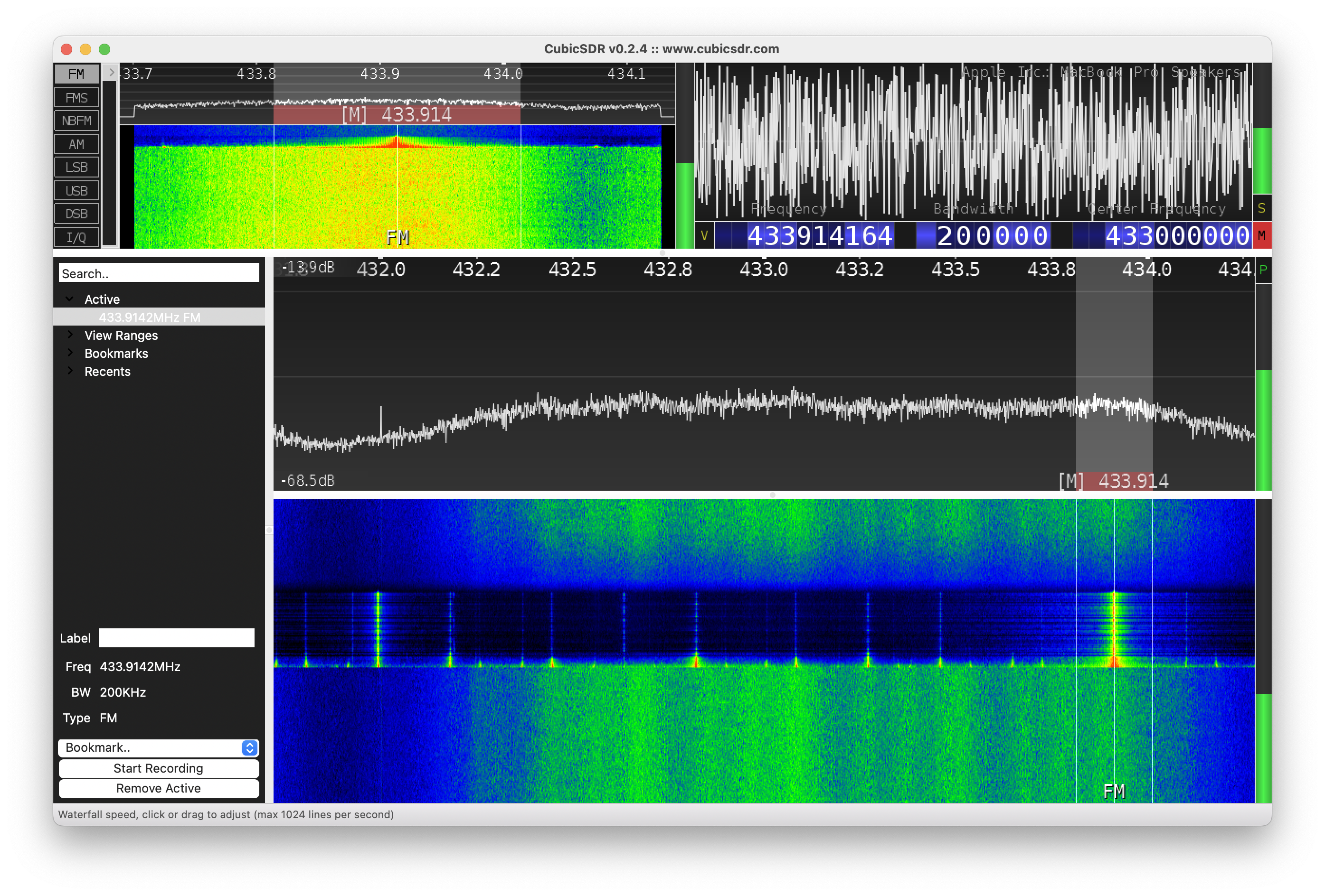
As predicted, the signal is transmitting on ~433.92 MHz, and as we can see it’s a quite long. Before going further, let’s check out the new application we discussed previously, but did not try yet – rtl_433. The main feature of that app that it has pre built libraries which can decode the signal “on air”. Let’s make a long story short and just launch rtl_433 following with the TX button pressing.
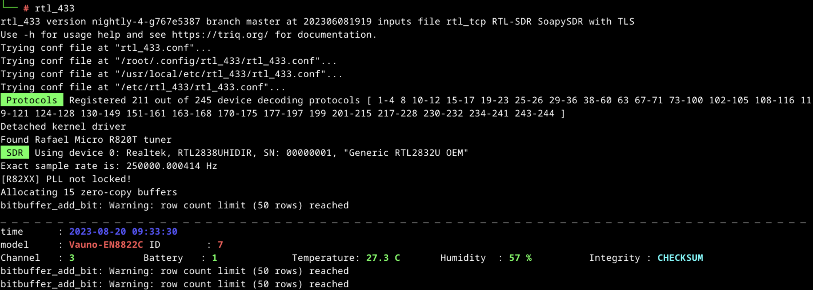
Great, we got it hence let’s analyze the data.
First of all, the model we are dealing with is Vauno-EN8822C. Simple Google request shows us plenty of stuff from that company including our weather station. Seems like the reseller in our case forgot to mention the origin name or, in a worst-case scenario, just “copy-pasted” the stuff.
Next, the Channel is 3, Battery – 1, Temperature – 27.3 C, Humidity -57%. The last one is the Checksum of Integrity.
Let’s compare harvested data with numbers on the original receiver:
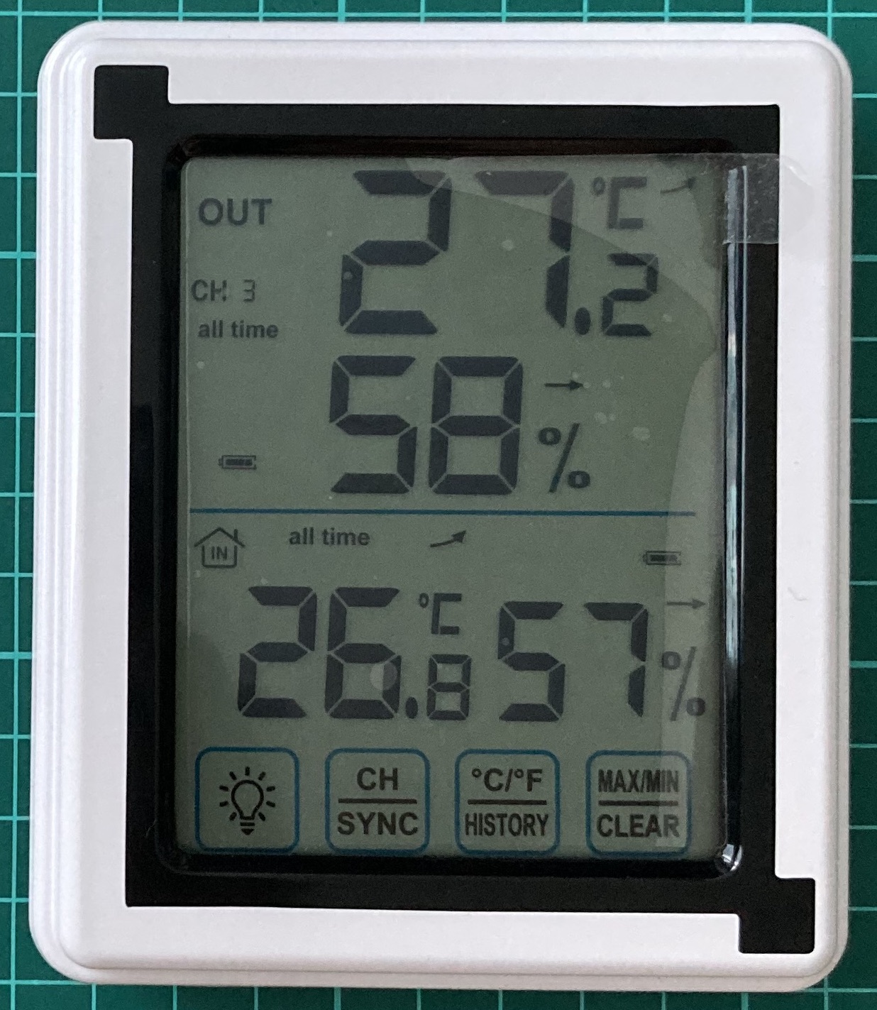
It’s almost accurate. Channel 3 is correct. Regarding battery we don’t know yet but due to the fact it’s full on the screen, we may predict that status 1 shows the full charge. Temperature is 27.3 against 27.2 which is fine. The humidity is 57 against 58 which is fine as well.
Before going deeper in reverse engineering and reading relative libraries, let’s try to think about what we have and the data we should receive.
At least there are 5 items (channel, battery, temperature, humidity and integrity) transmitted via radio waves. Based on previous experience we know that data is transmitting by 1 and 0 hence all numbers have to be decoded from decimal into binary.
Let’s start with the channel: it can be 1, 2 or 3 so there is no need to keep plenty space for it. The maximum number of the channel is 3 which is “10” in binary and it takes only 2 bits.
We may predict the same situation with the battery. If you look carefully at the receiver screen, you can see the battery divided into 2 pieces: the long one and the short one. We have already known the 1 is the full battery. We may assume the 2 as have battery and the 3 as the empty one. In that case the maximum number is 3 as well hence it could be “10” in binary and it takes only 2 bits as well.
Next is the temperature. The temperature by itself consists of 3 numbers: 2 numbers for the integer and 1 number for the float. In our case to get 27.2 C, we have to receive 272 which is 2 to the power of 9 (2^9) minus 240.
If we open the user manual, we can find the range of an outdoor temperature: from -40 C till 70 C. Keeping that in mind, overall, we have a 110-integer range. Don’t forget to multiply it by 10 to cover the float numbers as well. In total, the transmitter has to send 1100 different temperature ranges, which in binary is 2^11 (2048). The 2^10 (1024) is a little bit low and can’t cover the full scope.
The humidity. By the user manual it has 75% range: from 20% till 95%. Because it does not have the float number, 75 is the final range. The closest to it is 2^7 (128) because 2^6 (64) can’t cover the full scope.
Having combined that all together we have to get something simular to the below:
00 00 00000000000 0000000
At least there are 22 bits, but don’t forget about the integrity which can be additional 5-6 bits.
Ok, the brief theory is over and let’s apply it. We will open URH and get the signal.
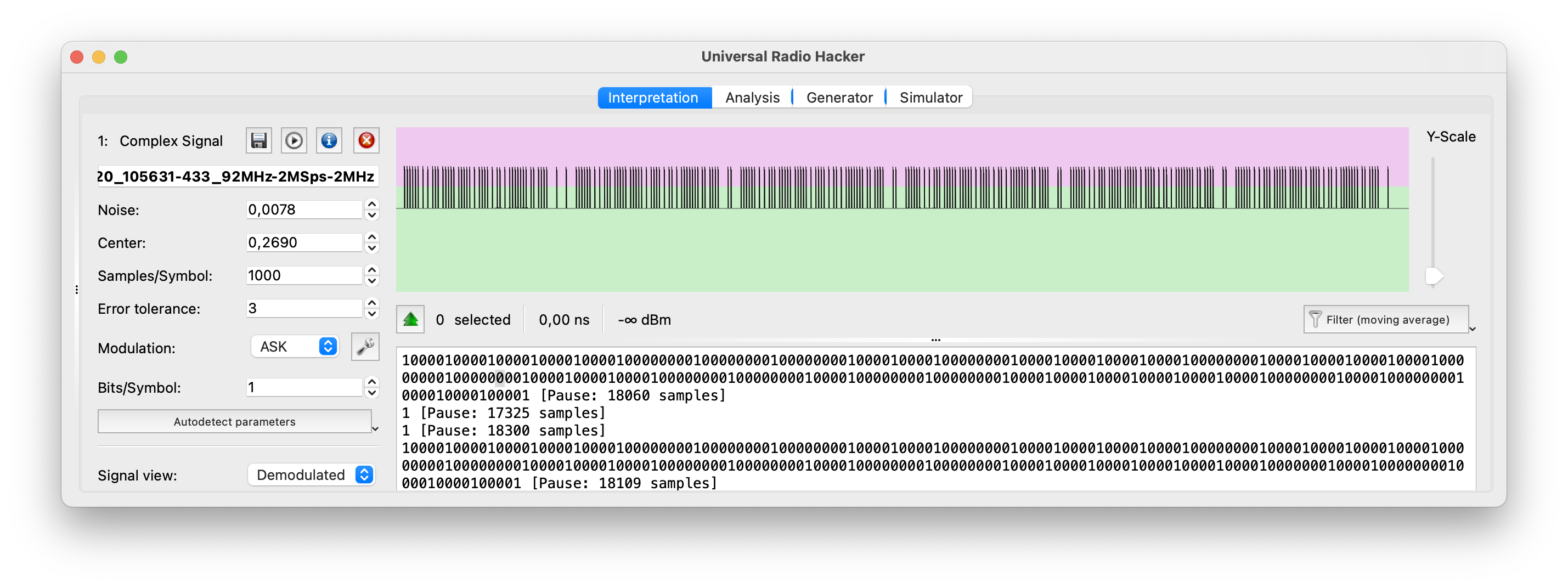
Hm, from the first view it seems scary – an excessive amount of data. But if we look closer, we may see the same data is repeating 6 times.
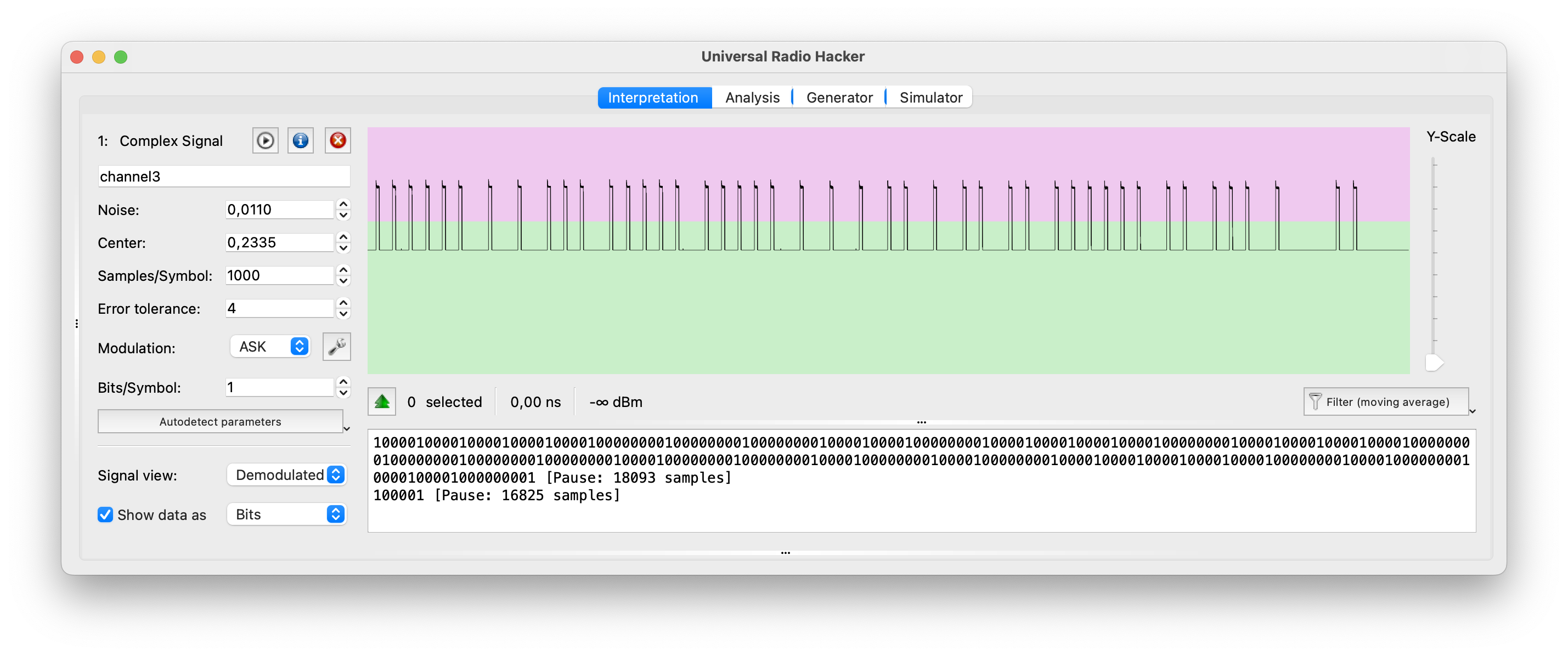
That’s much easier to analyze 🙂
First, let’s count the number of bits which are 262 (from peak to peak). But let’s keep in mind if we are talking about group of bits as one item (e.g. 1000), there could be plus 3-4 bits at the end.
Now it’s time for some experiments: let’s change the channel to 1 and 2 and catch the payload.
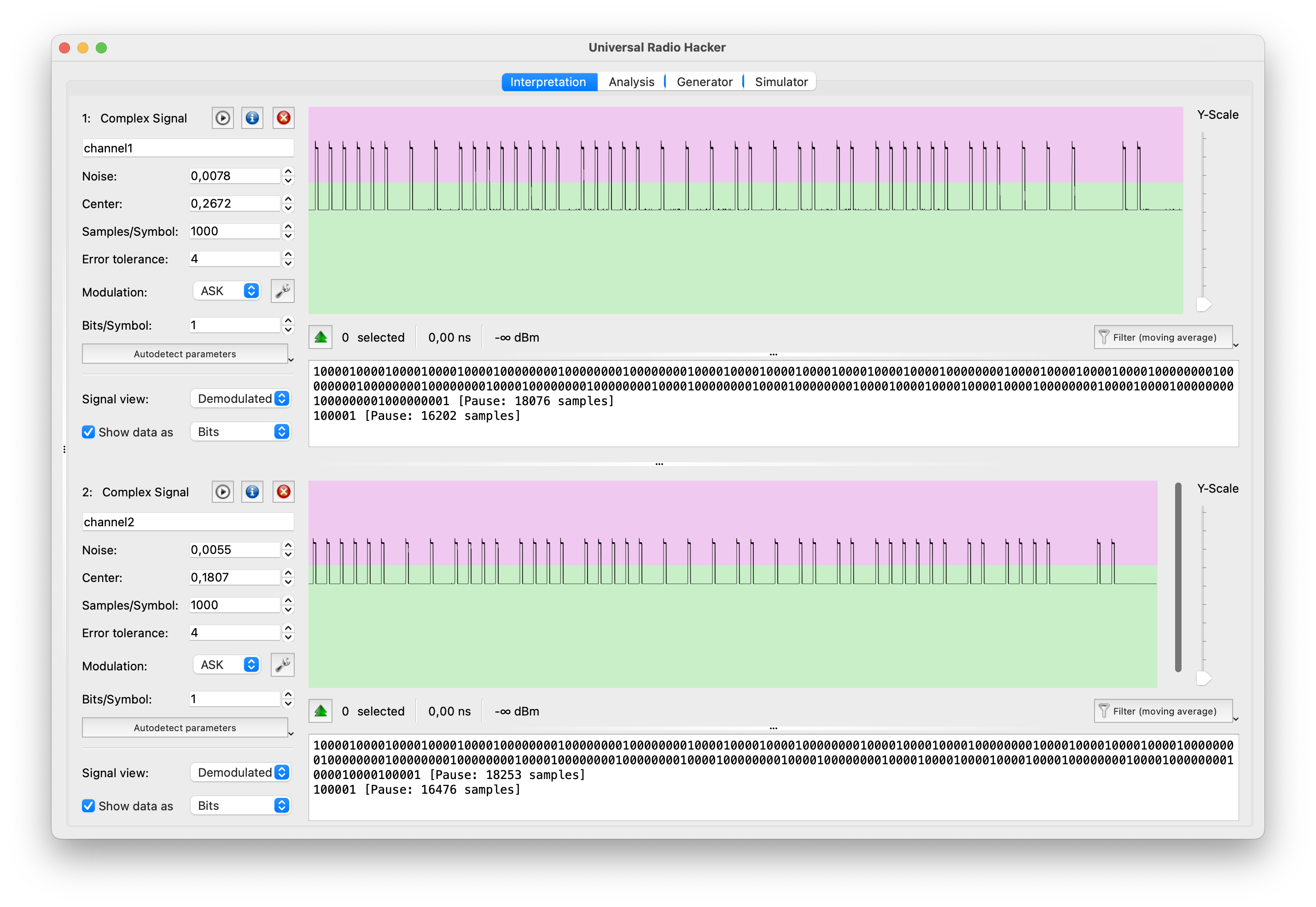
Great. Channel 1 (top) and 2 (bottom) have been well received and we can look at them.
We won’t look at repeated peaks because they can be whatever we can imagine hence let’s concentrate our eyes into the differences.
As you can mention, in channel 3 (first picture) the payload is 11011111 (if we consider the peak as 1, and the peak with pause as 0), channel 2 – 11101111 and the channel 1 – 11111111.
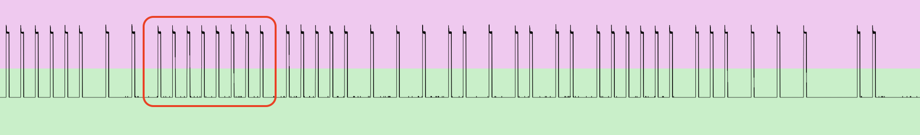
Great, what else we can get from here? Let’s look closer and try to find the pattern.
We may also say there are the exact number of peaks each payload, divided by pauses – 45 peaks. In that case we may suggest that 1 item is the short one – 10000, and 0 item is the long one – 100000000 or vice versa.
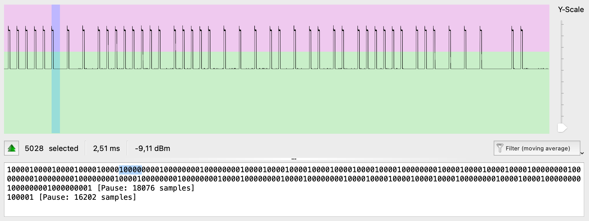
Also, let’s count the number of samples for each bit. In our case we have 275 bits (0’s and 1’s) with 285501 samples. Let’s divide those 2 numbers and find out the duration of each bit – 1038 samples.
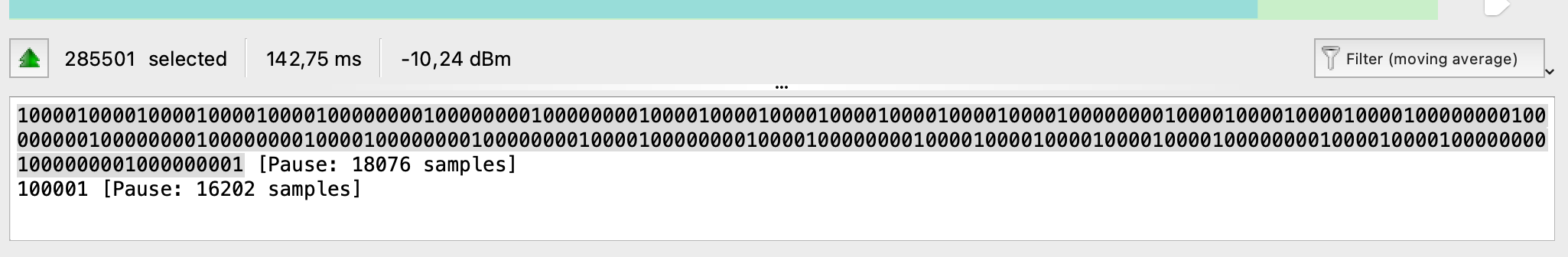
Great, what’s next? Next, we have to perform a deep research / reverse engineering: change the humidity, change the temperature, find old batteries and each time get the payload and see what is changing.
Hopefully for us, that research has already been done by rtl_433 application developers – https://github.com/merbanan/rtl_433/.
Let’s open the source code for our device and try to understand how it’s working – https://github.com/merbanan/rtl_433/blob/master/src/devices/vauno_en8822c.c.
Take a look at lines 21-33:
Frame structure (42 bits):
Byte: 0 1 2 3 4
Nibble: 1 2 3 4 5 6 7 8 9 10 11
Type: IIIIIIII B?CCTTTT TTTTTTTT HHHHHHHF FFFBXXXX XX
– I: Random device ID
– C: Channel (1-3)
– T: Temperature (Little-endian)
– H: Humidity (Little-endian)
– F: Flags (unknown)
– B: Battery (1=low voltage ~<2.5V)
– X: Checksum (6 bit nibble sum)
Each bit is explained in details. The most interesting part is that we were able to find the correct channel bits: bits order 11 and 12, just like we found.
Next, we have 12 bits for the temperature. Based on our calculations earlier, 11 is enough, but we guess the manufactory decided to round it up.
The humidity length is 7 bits just exact how many we calculated earlier.
Excellent, I guess we finished that hacking as well.
We hope that synthesizing the payload, knowing the pattern and how GNU Radio Companion working, won’t be a big problem to you hence it will be your homework. Play around with different temperatures and humidity and think how you can use it in real hacking.
But before we go, one more interesting detail about weather station.
C. Risk
What risk in hiding under using wireless weather station in your smart houses, work or OT environment?
Let us show you one interesting video – https://www.youtube.com/watch?v=L0fSEbGEY-Q
If you are reading that book offline and don’t have an internet connection, we will reveal the story in a nutshell.
In that video Mr. Andreas Spiess is building the smart device using RTL-SDR, Arduino and weather station with a wind measure.
So, the weather station is measuring the wind speed and wirelessly sending the data to the receiver. Using RTL-SDR he intercepts the signal and get the data including the wind speed. Depends on the speed, Arduino is sending signals to his outdoor awning – close it or open.
Now imagine that an angry hacker is living next to his house and they have a bad relationships. Knowing what Mr. Andreas has done, the hacker in a windy weather could spoof the legitimate signal and start sending payloads with a “good weather”. In that case Mr. Andreas’ outdoor awning could be seriously damaged.
Another case, if your employer is using wireless temperature measure for the server room: temperature is going up – switch on the AC, temperature is normal – switch off of decrease the power of AC.
In the worst-case scenario, following the save pattern like with Mr. Andreas, the whole company could be damaged significantly due to using a 25 dollars stuff.
11. Afterword
Definitely, it’s not the full scope of SDR hacking. We did not talk about car alarms and satellites hacking, GSM and GPS spoofing, rolling codes, and plenty of other stuff.
Drone landing, gamepad decoding and video intercepting are another valuable area of our common researches. We will definitely cover all of those aspects in our future articles and, maybe, in the Edition 2.
Please, share with us your thoughts and feedback regarding this article/book, what else you want to know and what areas should be revealed.
Nevertheless, if you need help, support or advice, please don’t hesitate to reach out to us using the contact information provided below.
Take care of your cyber hygiene.